Getting started tutorial part 6: analyzing measurement catalogs in multiple bands
In this part of the tutorial series you’ll analyze the forced photometry measurement catalogs you created in step 5. You’ll learn how to work with measurement tables and plot color-magnitude diagrams (CMDs).
Set up
Pick up your shell session where you left off in part 5.
That means your current working directory must contain the DATA directory (the Butler repository).
The lsst_distrib package also needs to be set up in your shell environment.
See Setting up installed LSST Science Pipelines for details on doing this.
As in part 3, you’ll be working inside an interactive Python session for this tutorial. You can use the default Python shell (python), the IPython shell, or even run from a Jupyter Notebook. Ensure that this Python session is running from the shell where you ran setup lsst_distrib.
Loading forced photometry measurement catalogs with the Butler
The forcedPhotCoadd.py command-line task (Running Forced photometry on coadds) created deepCoadd_forced_src datasets for each coadd in the example data repository.
Being forced photometry catalogs, rows in each deepCoadd_forced_src table correspond row-for-row across all coadds in different filters for a sky map patch.
Since you don’t have to do additional cross-matching, these deepCoadd_forced_src datasets are convenient.
To get these datasets, open a Python session (IPython or Jupyter Notebook) and create a Butler:
import lsst.daf.persistence as dafPersist
butler = dafPersist.Butler(inputs='DATA/rerun/coaddForcedPhot')
This Butler is using the coaddForcedPhot rerun you created for the forcePhotCoadd.py command-line task’s outputs.
Next, use the Butler to get the deepCoadd_forced_src datasets for both filters:
rSources = butler.get('deepCoadd_forced_src', {'filter': 'HSC-R', 'tract': 0, 'patch': '1,1'})
iSources = butler.get('deepCoadd_forced_src', {'filter': 'HSC-I', 'tract': 0, 'patch': '1,1'})
These datasets correspond to coadds for a single patch (1,1 in tract 0) for both the HSC-R and HSC-I filters.
Getting calibrated PSF photometry
The base_PsfFlux_flux column of these deepCoadd_forced_src datasets is the flux from the linear least-squares fit of the PSF model to the source.
From the source table’s schema you know this flux has units of counts:
iSources.getSchema().find('base_PsfFlux_flux').field.getUnits()
Transforming this flux into a magnitude requires knowing the coadd’s zeropoint, which you can get from the coadd dataset.
The coadd you made in part 4 with assembleCoadd.py doesn’t have calibration info attached to it, though.
Instead, you want the deepCoadd_calexp dataset, which was created by the detectCoaddSources.py command-line task, because it does have calibrations.
You can access these calibrations directly from deepCoadd_calexp_calib datasets for each filter:
rCoaddCalib = butler.get('deepCoadd_calexp_calib',  {'filter': 'HSC-R', 'tract': 0, 'patch': '1,1'})
iCoaddCalib = butler.get('deepCoadd_calexp_calib',  {'filter': 'HSC-I', 'tract': 0, 'patch': '1,1'})
Note
An alternative way to get the lsst.afw.image.calib.Calib object is from the deepCoadd_calexp dataset object:
rCoaddCalexp = butler.get('deepCoadd_calexp',  {'filter': 'HSC-R', 'tract': 0, 'patch': '1,1'})
rCoaddCalib = rCoaddCalexp.getCalib()
These Calib objects not only have methods for directing accessing calibration information, but also for applying those calibrations.
Use the Calib.getMagnitude() method to transform fluxes in counts to magnitudes in the HSC instrument’s system (AB magnitudes):
rCoaddCalib.setThrowOnNegativeFlux(False)
iCoaddCalib.setThrowOnNegativeFlux(False)

rMags = rCoaddCalib.getMagnitude(rSources['base_PsfFlux_flux'])
iMags = iCoaddCalib.getMagnitude(iSources['base_PsfFlux_flux'])
Note
The reason you called the Calib.setThrowOnNegativeFlux method was to prevent an exception from being raised for sources with negative fluxes.
This is commonly required for forced photometry analysis since some sources may not be visible in a band so that the flux measurement is effectively of blank sky.
Because of background variance, the measured flux of non-detections can be randomly negative.
Filtering for unique, deblended sources with the detect_isPrimary flag
Before going ahead and plotting a CMD from the full source table, you’ll typically need to do some basic filtering. Exactly what filtering is done depends on the application, but source tables should always be filtered for unique sources. There are two ways that measured sources might not be unique: deblended sources, and sources in patch overlaps.
Finding deblended sources
When objects are detected, they are deblended.
Deblending involves decomposing a source into multiple child sources that have local flux peaks.
In source tables like rSources and iSources, both the original (blended) and de-blended sources are included in the table.
This is done so that you can choose whether to use blended or deblended measurements in your analysis.
If you don’t choose, though, the same flux will be included multiple times in your analysis.
Usually you will want to use fully-deblended sources in your analysis.
The best way to identify fully-deblended sources is those that have no children (children being sources deblended from that parent source) given the deblend_nChild column.
Make a boolean index array of deblended sources:
deblended = rSources['deblend_nChild'] == 0
Finding primary detections
The other reason a source in the table might not be unique is if it falls in the overlaps of patches. Sources in overlaps appear in multiple measurement tables.
If you are analyzing multiple patches, or multiple tracts, you want to use the primary detection for each source. The Pipelines determine if a detection in a patch is primary, or not, by whether it falls in the inner region of that patch (and tract). An inner region is a part of a sky map exclusively claimed by one patch.
The flag that indicates whether a source lies in the patch’s inner region isn’t in the deepCoadd_forced_src table though.
Instead, you need to look at the deepCoadd_ref table made by mergeCoaddMeasurements.py in the previous tutorial.
Begin by using the Butler to get the deepCoadd_ref dataset for patch you’re analyzing:
refTable = butler.get('deepCoadd_ref', {'filter': 'HSC-R^HSC-I', 'tract': 0, 'patch': '1,1'})
Then make an index array from the combination of detect_isPatchInner and detect_isTractInner flags:
inInnerRegions = refTable['detect_isPatchInner'] & refTable['detect_isTractInner']
The go-to flag: detect_isPrimary
You actually want the combination of the isDeblended and inInnerRegions arrays you just made.
The deepCoadd_ref table provides a shortcut for this: the detect_isPrimary flag identifies sources that are both fully deblended and in inner regions.
Run:
isPrimary = refTable['detect_isPrimary']
Now you can use this array to slice the photometry arrays and get only primary sources, like this:
rMags[isPrimary]
iMags[isPrimary]
Note
The detect_isPrimary flag is defined by this algorithm:
(deblend_nChild == 0) & detect_isPatchInner & detect_isTractInner
Tip
You can learn about any table column from the schema. For example:
refTable.schema.find('detect_isPrimary')
You can get a list of all columns available in a table by running:
refTable.schema.getNames()
Quickly classifying stars and galaxies
Reliably classifying sources as stars and galaxies is not easy, but you can get a rough estimate based on the extendedness of sources.
The base_ClassificationExtendedness_value column is 1. for extended sources (galaxies) and 0. for point sources (like stars).
To see this for yourself, run:
iSources.schema.find('base_ClassificationExtendedness_value').field.getDoc()
Go ahead and create a boolean index of sources classified as point sources:
isStellar = iSources['base_ClassificationExtendedness_value'] < 1.
Using measurement flags
Lastly, you may want to work with only high-quality measurements.
Earlier, you got PSF fluxes of sources (base_PsfFlux_flux).
The base_PsfFlux measurement plugin also creates flags that describe measurement errors and issues.
You can find these flags, as usual, from the table schema.
Here’s a way to find columns produced by the base_PsfFlux plugin:
iSources.getSchema().extract('base_PsfFlux_*')
A useful flag is base_PsfFlux_flag, which is the logical combination of specific base_PsfFlux error flags:
isGoodFlux = ~iSources['base_PsfFlux_flag']
Since the base_PsfFlux_flag is True for sources with measurement errors, you used the unary invert operator (~) so that well-measured sources are True in the isGoodFlux array.
Finally, combine all these boolean index arrays together:
selected = isPrimary & isStellar & isGoodFlux
In the next step, you’ll plot a color-magnitude diagram of the sources you’ve selected.
Plot a CMD
The product of this effort will be an r-i CMD. You can use matplotlib to create this visualization:
import matplotlib.pyplot as plt

plt.style.use('seaborn-notebook')
plt.figure(1, figsize=(4, 4), dpi=140)
plt.scatter(rMags[selected] - iMags[selected],
            iMags[selected],
            edgecolors='None', s=2, c='k')
plt.xlim(-0.5, 3)
plt.ylim(25, 14)
plt.xlabel('$r-i$')
plt.ylabel('$i$')
plt.subplots_adjust(left=0.125, bottom=0.1)
plt.show()
You should see a figure like this:
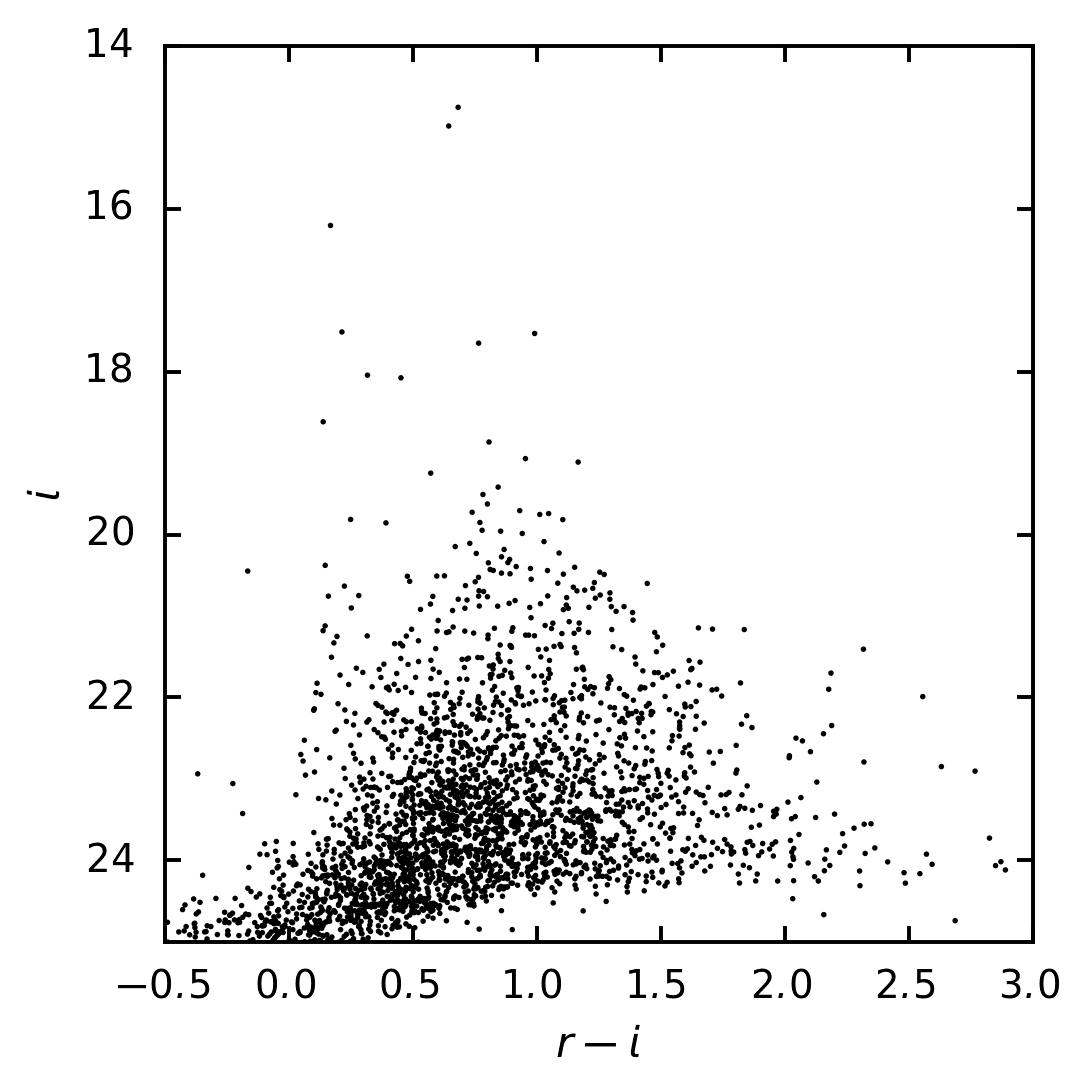
r-i color-magnitude diagram of stars.
Wrap up
In this tutorial, you gained experience working with source measurement catalogs created by the LSST Science Pipelines. Here are some takeaways:
- Forced photometry source tables are
deepCoadd_forced_srcdatasets. They’re convenient to use becausedeepCoadd_forced_srctables from different filters (for a given sky map patch) correspond row-for-row. - You need to filter sources for uniqueness due to deblending and patch overlaps.
The
detect_isPrimarycolumn from thedeepCoadd_refdataset is the go-to flag for doing this. - Use the
base_ClassificationExtendedness_valuecolumn to quickly distinguish stars from galaxies. - The
base_PsfFlux_flagcolumn is useful for identifying sources that don’t have photometric measurement errors.
In the end, you created a simple r-i CMD.
This tutorial is just the beginning, though.
With the dataset you’ve created in this tutorial, you can look at galaxies with measurements from the CModel plugin.
Or compare PSF-fitted photometric measurements with aperture photometry of stars.
When you’re ready, dive into the rest of the LSST Science Pipelines documentation to begin processing your own data. As you’re learning, don’t hesitate to reach out with questions on the LSST Community forum.