ColorColorFitPlot

class lsst.analysis.tools.actions.plot.ColorColorFitPlot(*args, **kw)

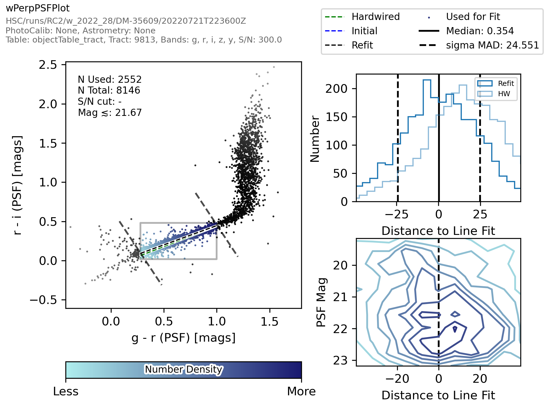
Bases: PlotAction

Makes a color-color plot and overplots a prefited line to the specified area of the plot. This is mostly used for the stellar locus plots and also includes panels that illustrate the goodness of the given fit.

Attributes Summary

magLabel	Label to use for the magnitudes used to color code by (str)
minPointsForFit	Minimum number of valid objects to bother attempting a fit.
plotName	The name for the plot.
plotTypes	Selection of types of objects to plot.
xAxisLabel	Label to use for the x axis (str)
yAxisLabel	Label to use for the y axis (str)

Methods Summary

__call__(data, **kwargs)	Call self as a function.
getInputSchema(**kwargs)	Return the schema an AnalysisAction expects to be present in the arguments supplied to the __call__ method.
makePlot(data, plotInfo, **kwargs)	Make stellar locus plots using pre fitted values.

Attributes Documentation

magLabel

Label to use for the magnitudes used to color code by (str)

minPointsForFit

Minimum number of valid objects to bother attempting a fit. (int, default 5)

Valid Range = [1,inf)

plotName

The name for the plot. (str)

plotTypes

Selection of types of objects to plot. Can take any combination of stars, galaxies, unknown, mag, any. (List, default ['stars'])

xAxisLabel

Label to use for the x axis (str)

yAxisLabel

Label to use for the y axis (str)

Methods Documentation

__call__(data: MutableMapping[str, ndarray[Any, dtype[ScalarType]] | Scalar | HealSparseMap], **kwargs) → Mapping[str, Figure] | Figure

Call self as a function.

getInputSchema(**kwargs) → HealSparseMap]]]

Return the schema an AnalysisAction expects to be present in the arguments supplied to the __call__ method.

Returns:

resultKeyedDataSchema

The schema this action requires to be present when calling this action, keys are unformatted.

makePlot(data: MutableMapping[str, ndarray[Any, dtype[ScalarType]] | Scalar | HealSparseMap], plotInfo: Mapping[str, str], **kwargs) → Figure

Make stellar locus plots using pre fitted values.

Parameters:

dataKeyedData

The data to plot the points from, for more information please see the notes section.

plotInfodict

A dictionary of information about the data being plotted with keys:

• "run"

  The output run for the plots (str).

• "skymap"

  The type of skymap used for the data (str).

• "filter"

  The filter used for this data (str).

• "tract"

  The tract that the data comes from (str).

Returns:

figmatplotlib.figure.Figure

The resulting figure.

Notes

The axis labels are given by self.config.xLabel and self.config.yLabel. The perpendicular distance of the points to the fit line is given in a histogram in the second panel.

For the code to work it expects various quantities to be present in the ‘data’ that it is given.

The quantities that are expected to be present are:

• Statistics that are shown on the plot or used by the plotting code:

  • approxMagDepth

    The approximate magnitude corresponding to the SN cut used.

  • f"{self.plotName}_sigmaMAD"

    The sigma mad of the distances to the line fit.

  • f"{self.identity or ''}_median"

    The median of the distances to the line fit.

  • f"{self.identity or ''}_hardwired_sigmaMAD"

    The sigma mad of the distances to the initial fit.

  • f"{self.identity or ''}_hardwired_median"

    The median of the distances to the initial fit.

• Parameters from the fitting code that are illustrated on the plot:

  • "bHW"

    The hardwired intercept to fall back on.

  • "bODR"

    The intercept calculated by the orthogonal distance regression fitting.

  • "bODR2"

    The intercept calculated by the second iteration of orthogonal distance regression fitting.

  • "mHW"

    The hardwired gradient to fall back on.

  • "mODR"

    The gradient calculated by the orthogonal distance regression fitting.

  • "mODR2"

    The gradient calculated by the second iteration of orthogonal distance regression fitting.

  • "xMin`"

    The x minimum of the box used in the fit.

  • "xMax"

    The x maximum of the box used in the fit.

  • "yMin"

    The y minimum of the box used in the fit.

  • "yMax"

    The y maximum of the box used in the fit.

  • "mPerp"

    The gradient of the line perpendicular to the line from the second ODR fit.

  • "bPerpMin"

    The intercept of the perpendicular line that goes through xMin.

  • "bPerpMax"

    The intercept of the perpendicular line that goes through xMax.

• The main inputs to plot:

  x, y, mag

Examples

An example of the plot produced from this code is here:

For a detailed example of how to make a plot from the command line please see the getting started guide.