

Inject Synthetic Sources#
Injecting Synthetic Sources Into Visit-Level or Coadd-Level Dataset Types#
Synthetic sources can be injected into any imaging data product output by the LSST Science Pipelines. This is useful for testing algorithmic performance on simulated data, where the truth is known, and for subsequent quality assurance tasks.
The sections below describe how to inject synthetic sources into a visit-level exposure-type or visit-type datasets (i.e., datasets with the dimension exposure or visit), or into a coadd-level dataset.
Options for injection on the command line and in Python are presented.
Prior to injection, the instructions on this page assume that the user will already have in-place a fully qualified source injection pipeline definition YAML (see Make an Injection Pipeline) and a suitable synthetic source injection catalog describing the sources to be injected (see Generate an Injection Catalog) which has been ingested into the data butler (see Ingest an Injection Catalog).
Injection on the Command Line#
Source injection on the command line is performed using the pipetask run command.
The process for injection into visit-level imaging (i.e., exposure or visit type data) or injection into coadd-level imaging (e.g., a deep_coadd_predetection`) is largely the same, save for the use of a different data query and a different injection task or pipeline subset.
The following command line example injects synthetic sources into the LSST exposure 2025050300351 detector 94 post_isr_image dataset.
For the purposes of this example we run the isr, injectExposure and calibrateImage tasks.
These tasks will process raw science data through to preliminary visit-level calibrated output imaging.
The injectExposure task (:lsst-task:`~lsst.source.injection.ExposureInjectTask`) has been merged into a reference pipeline following a successful run of make_injection_pipeline, with neighboring task connections modified to account for source injection.
Tip
Injection into a coadd-level data product such as a deep_coadd_predetection can easily be achieved by generating a new injection pipeline, substituting injectExposure for injectCoadd in the list of tasks being run, and modifying the -d data query.
For the injection catalog generated in these notes, this coadd-level data query would work well:
-d "instrument='LSSTCam' AND skymap='lsst_cells_v1' AND tract=10321 AND patch=66 AND band='r'"
pipetask --long-log --log-file $LOGFILE \
run --register-dataset-types \
-b $REPO \
-i $INPUT_DATA_COLL,$INJECTION_CATALOG_COLL \
-o $OUTPUT_COLL \
-p DRP-injection.yaml#isr,injectExposure,calibrateImage \
-d "instrument='LSSTCam' AND exposure=2025050300351 AND detector=94"
where
$LOGFILEThe full path to a user-defined output log file.
$REPOThe path to the butler repository.
$INPUT_DATA_COLLThe name of the input data collection.
$INJECTION_CATALOG_COLLThe name of the input injection catalog collection.
$OUTPUT_COLLThe name of the injected output collection.
Caution
Standard processing should not normally have to make use of the --register-dataset-types flag.
This flag is only required to register a new output dataset type with the butler for the very first time.
If injection outputs have already been generated within your butler repository, you should omit this flag from your run command to prevent any accidental registration of unwanted dataset types.
Note
Existing subsets will have injection variants denoted by the prefix injected_.
These subsets include the injection task and any tasks after the point of source injection.
The injected_ subsets can save memory and runtime if the tasks prior to injection have already been run.
The image plane of the injected_post_isr_image will be modified from the original by the addition of a light profile for every injected object.
By default the injected light profiles have simulated shot noise added. This can be turned off by setting add_noise to False in the injection task config.
The variance plane gains additional estimated variance consistent with the amount of light added to the image plane, including any simulated noise.
Caution
Setting inject_variance to False in the injection task config will prevent any changes to the variance plane.
Not modifying the variance plane is likely to bias any downstream measurements and should normally never be done, unless such bias is the object of study.
Assuming processing completes successfully, the injected_post_isr_image and associated injected_post_isr_image_catalog will be written to the butler repository (see example images below).
Standard log messages that get printed as part of a successful run may include lines similar to:
Retrieved 216 injection sources from 3 HTM trixels.
Identified 99 injection sources with centroids outside the padded image bounding box.
Catalog cleaning removed 99 of 216 sources; 117 remaining for catalog checking.
Catalog checking flagged 0 of 117 sources; 117 remaining for source generation.
Adding INJECTED and INJECTED_CORE mask planes to the exposure.
Generating 117 injection sources consisting of 1 unique type: Sersic(117).
Injected 117 of 117 potential sources. 0 sources flagged and skipped.
An example injected output produced by the above snippet is shown below.

Calibrated exposure data for LSSTCam visit 2025050300351, detector 94, showcasing the injection of a series of synthetic Sérsic sources before and after injection. Images are asinh scaled.
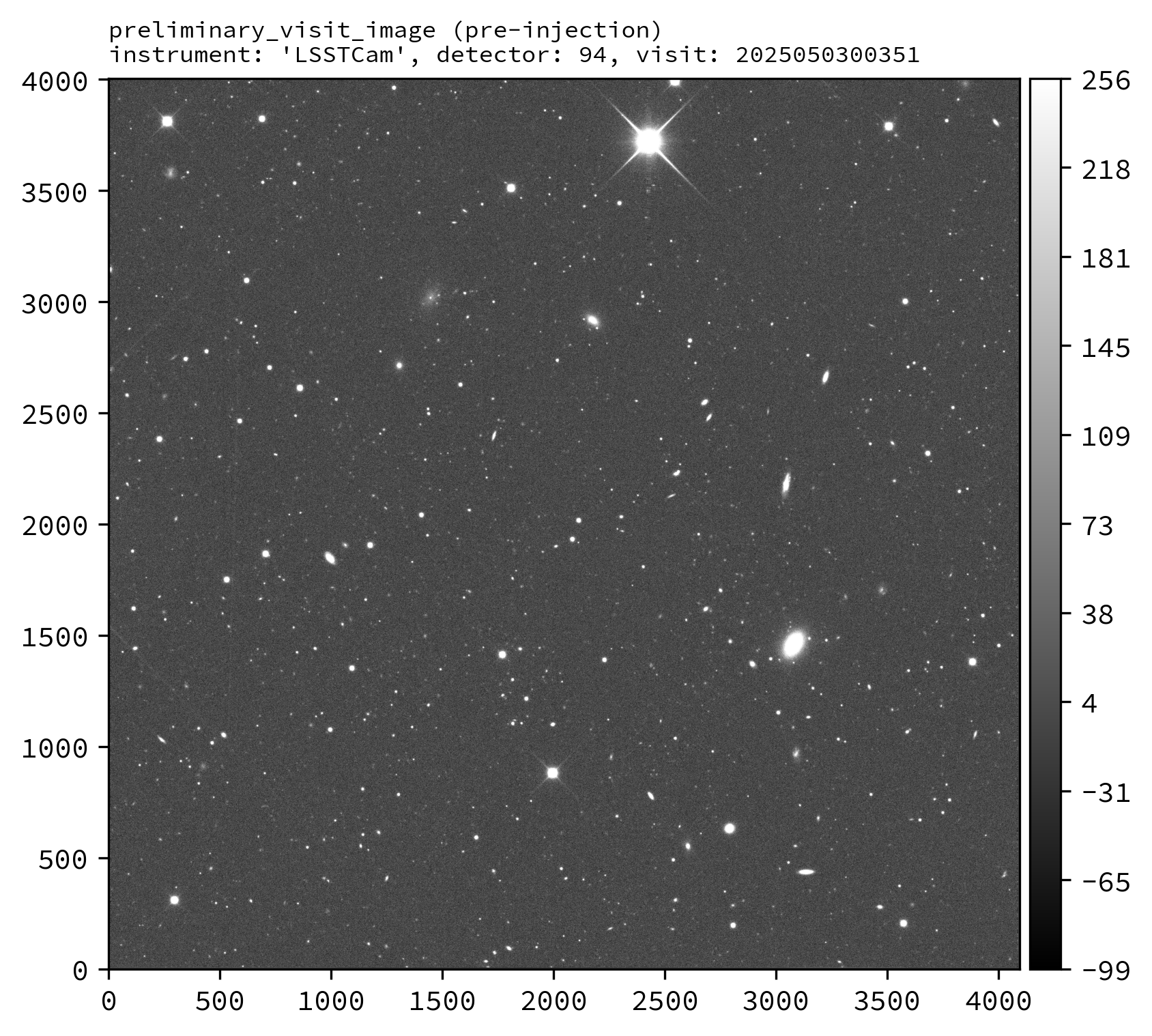
Before injection. |
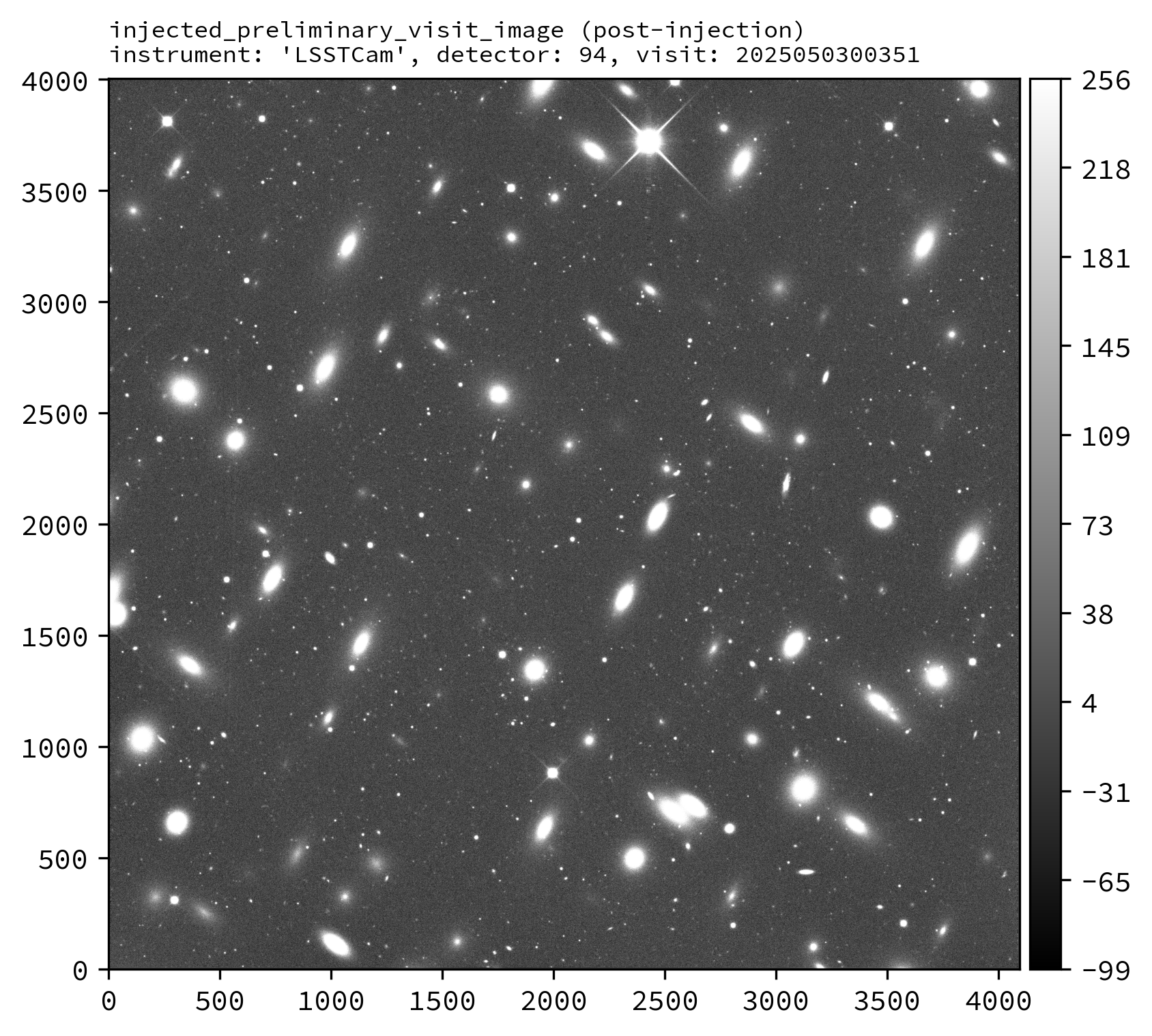
After injection. |
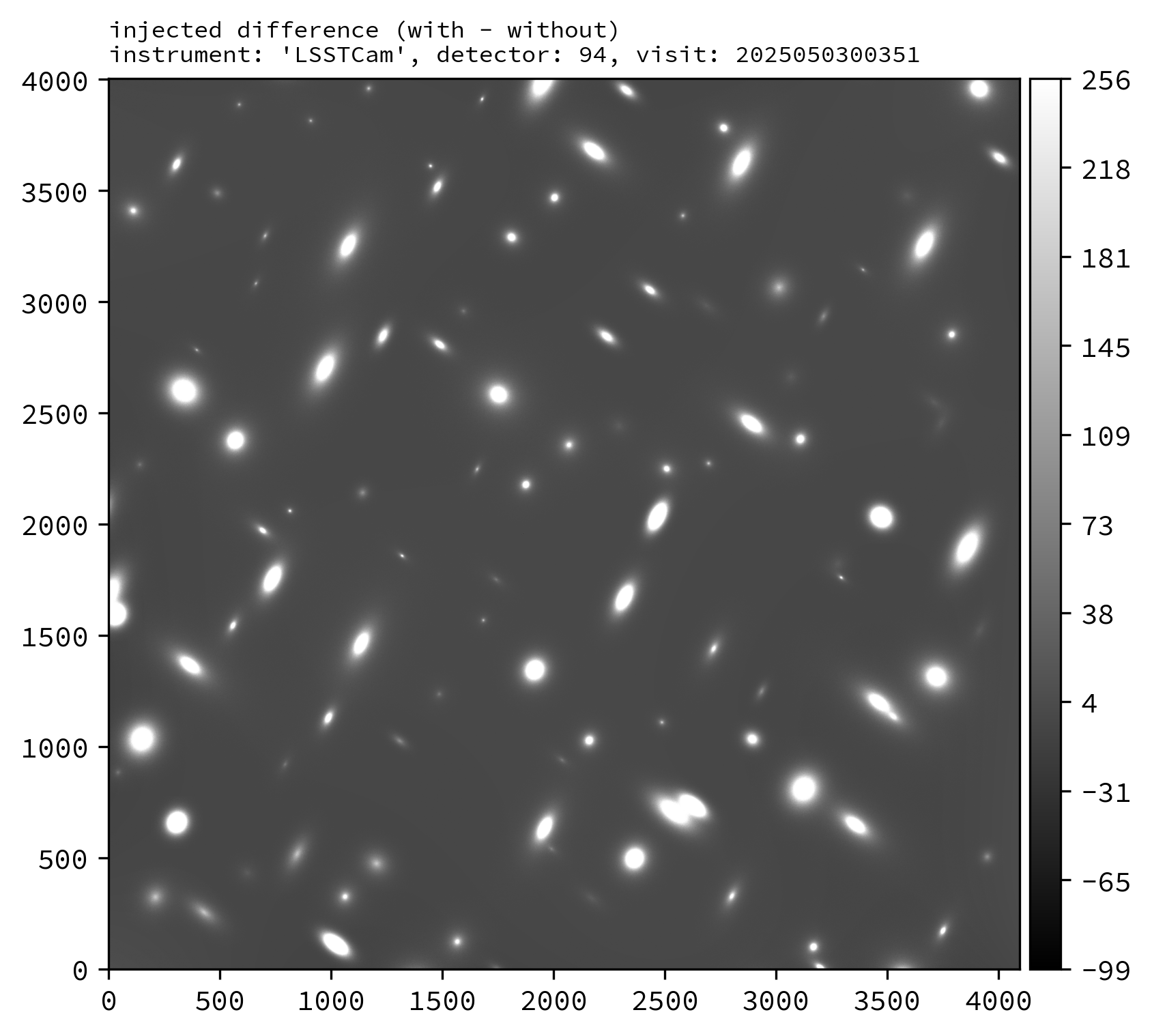
Difference image. |
Injection in Python#
Source injection in Python is achieved by calling the source injection task classes directly. As on the command line, the process for injection into visit-level imaging or coadd-level imaging is largely the same, save for the use of a different task class, a different data query, and use of different calibration data products (see the notes in the Python snippet below).
The following Python example injects synthetic sources into the LSSTCam r-band tract 10321 patch 66 deep_coadd_predetection dataset.
For the purposes of this example, we will just run the source injection task alone.
from lsst.daf.butler import Butler
from lsst.source.injection import CoaddInjectConfig, CoaddInjectTask

# NOTE: For injections into other dataset types, use the following instead:
# from lsst.source.injection import ExposureInjectConfig, ExposureInjectTask
# from lsst.source.injection import VisitInjectConfig, VisitInjectTask

# Instantiate a butler.
butler = Butler.from_config(REPO)

# Load an input coadd dataset.
dataId = dict(
    instrument="LSSTCam",
    skymap="lsst_cells_v1",
    tract=10321,
    patch=66,
    band="r",
)
input_exposure = butler.get(
    "deep_coadd_predetection",
    dataId=dataId,
    collections=INPUT_DATA_COLL,
)
# NOTE: Visit-level injections also require a visit summary table.
# visit_summary = butler.get(
#     "visit_summary",
#     dataId=dataId,
#     collections=INPUT_DATA_COLL,
# )

# Get calibration data products.
psf = input_exposure.getPsf()
photo_calib = input_exposure.getPhotoCalib()
wcs = input_exposure.getWcs()
# NOTE: Visit-level injections should instead use the visit summary table.
# detector_summary = visit_summary.find(dataId["detector"])
# psf = detector_summary.getPsf()
# photo_calib = detector_summary.getPhotoCalib()
# wcs = detector_summary.getWcs()

# Load input injection catalogs, here just for r-band catalogs.
injection_refs = butler.registry.queryDatasets(
    "injection_catalog",
    band="r",
    collections=INJECTION_CATALOG_COLL,
)
injection_catalogs = [butler.get(injection_ref) for injection_ref in injection_refs]

# Instantiate the injection classes.
inject_config = CoaddInjectConfig()
inject_task = CoaddInjectTask(config=inject_config)

# Run the source injection task.
injected_output = inject_task.run(
    injection_catalogs=injection_catalogs,
    input_exposure=input_exposure.clone(),
    psf=psf,
    photo_calib=photo_calib,
    wcs=wcs,
)
injected_exposure = injected_output.output_exposure
injected_catalog = injected_output.output_catalog
where
REPOThe path to the butler repository.
INPUT_DATA_COLLThe name of the input data collection.
INJECTION_CATALOG_COLLThe name of the input injection catalog collection.
An example injected output produced by the above snippet is shown below.
Coadd-level (deep_coadd_predetection and injected_deep_coadd_predetection) data for LSSTCam tract 10321, patch 66 in the r-band, showcasing the injection of a series of synthetic Sérsic sources.
Images are log scaled.
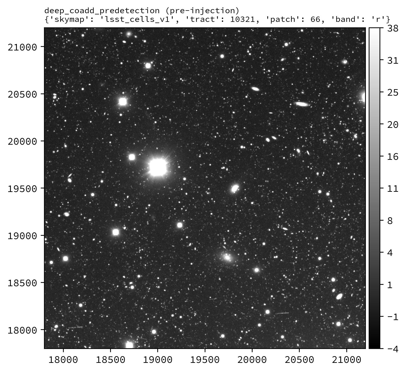
Before injection. |

After injection. |
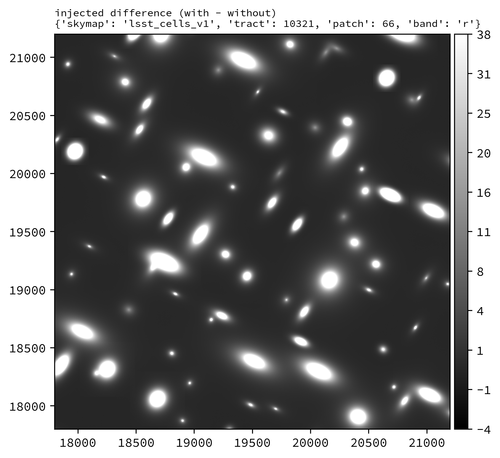
Difference image. |
Injecting Postage Stamps#
The commands above have focussed on injecting synthetic parametric models produced by GalSim. It’s also possible to inject FITS postage stamps directly into the data. These may be real astronomical images, or they may be simulated images produced by other software.
By way of example, lets inject multiple copies of the SDSS galaxy J122240.63+053053.6, a \(z\sim0.07\) galaxy of brightness \(m_{r}\sim17.6\) mag located in lsst_cells_v1 tract 10321, patch 66.
First, lets construct a small postage stamp using existing LSSTCam data products:
from lsst.daf.butler import Butler
from lsst.geom import Box2I, Extent2I, Point2I

# Instantiate a butler.
butler = Butler.from_config(REPO)

# Get the deep_coadd_predetection for LSSTCam r-band tract 10321, patch 66.
dataId = dict(
    instrument="LSSTCam",
    skymap="lsst_cells_v1",
    tract=10321,
    patch=66,
    band="r",
)
coadd = butler.get(
    "deep_coadd_predetection",
    dataId=dataId,
    collections=INPUT_DATA_COLL,
)

# Find the x/y coordinates for the galaxy.
wcs = coadd.wcs
x0, y0 = wcs.skyToPixelArray(185.6693295, 5.5149062, degrees=True)

# Create a 107x107 pixel postage stamp centered on the galaxy.
bbox = Box2I(Point2I(x0, y0), Extent2I(1,1))
bbox.grow(53)
stamp = coadd[bbox]

# Save the postage stamp image to a FITS file.
stamp.image.writeFits(POSTAGE_STAMP_FILE)
where
REPOThe path to the butler repository.
INPUT_DATA_COLLThe name of the input data collection.
POSTAGE_STAMP_FILEThe file name for the postage stamp FITS file.
This postage stamp looks like this:
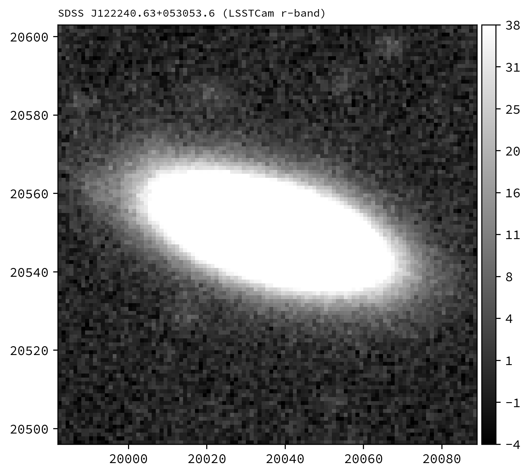
An LSSTCam r-band postage stamp of the SDSS galaxy J122240.63+053053.6, a \(z\sim0.07\) galaxy of brightness \(m_{r}\sim17.6\) mag located in LSSTCam tract 10321, patch 66. Image is log scaled.
Next, lets construct a simple injection catalog and ingest it into the butler.
Injection of FITS-file postage stamps only requires the ra, dec, source_type, mag and stamp columns to be specified in the injection catalog.
Note that below we switch from Python to the command line interface:
generate_injection_catalog \
-a 185.51 185.95 \
-d 5.33 5.56 \
-n 50 \
-p source_type Stamp \
-p mag 17.2 \
-p stamp $POSTAGE_STAMP_FILE \
-b $REPO \
-w deep_coadd \
-c $INPUT_DATA_COLL \
--where "instrument='LSSTCam' AND skymap='lsst_cells_v1' AND tract=10321 AND patch=66 AND band='r'" \
-i r \
-o $INJECTION_CATALOG_COLL
where
$POSTAGE_STAMP_FILEThe file name for the postage stamp FITS file.
$REPOThe path to the butler repository.
$INPUT_DATA_COLLThe name of the input data collection.
$INJECTION_CATALOG_COLLThe name of the input injection catalog collection.
The first several rows from the injection catalog produced by the above snippet look like this:
injection_id         ra                dec         source_type mag           stamp
------------ ------------------ ------------------ ----------- ---- -----------------------
        0 185.62261633068604   5.51954052453572       Stamp 17.2 my_injection_stamp.fits
        1 185.54700111177948  5.471189971018477       Stamp 17.2 my_injection_stamp.fits
        2  185.8702087112494  5.391756668952863       Stamp 17.2 my_injection_stamp.fits
        3 185.78081900198586  5.408787617963841       Stamp 17.2 my_injection_stamp.fits
        4 185.71204589111636  5.445704245746881       Stamp 17.2 my_injection_stamp.fits
...
Finally, lets inject our postage stamp multiple times into the LSSTCam r-band tract 10321, patch 66 image:
pipetask --long-log --log-file $LOGFILE \
run --register-dataset-types \
-b $REPO \
-i $INPUT_DATA_COLL,$INJECTION_CATALOG_COLL \
-o $OUTPUT_COLL \
-p $SOURCE_INJECTION_DIR/pipelines/inject_coadd.yaml \
-d "instrument='LSSTCam' AND skymap='lsst_cells_v1' AND tract=10321 AND patch=66 AND band='r'" \
-c injectCoadd:stamp_prefix=$MY_INJECTION_STAMP_DIR
where
$LOGFILEThe full path to a user-defined output log file.
$REPOThe path to the butler repository.
$INPUT_DATA_COLLThe name of the input data collection.
$INJECTION_CATALOG_COLLThe name of the input injection catalog collection.
$OUTPUT_COLLThe name of the injected output collection.
$SOURCE_INJECTION_DIRThe path to the source injection package directory.
$MY_INJECTION_STAMP_DIRThe directory where the injection FITS file is stored.
Tip
If the injection FITS file is not in the same directory as the working directory where the pipetask run command is run, the stamp_prefix configuration option can be used as shown here.
This appends a string to the beginning of the FITS file name taken from the catalog, allowing for your FITS files to be stored in a different directory to the current working directory.
Running the above snippet produces the following:
Coadd-level (deep_coadd_predetection and injected_deep_coadd_predetection) data for LSSTCam tract 10321, patch 66 in the r-band, showcasing the injection of multiple copies of a postage stamp.
Images are log scaled.
|
Before injection. |

After injection. |
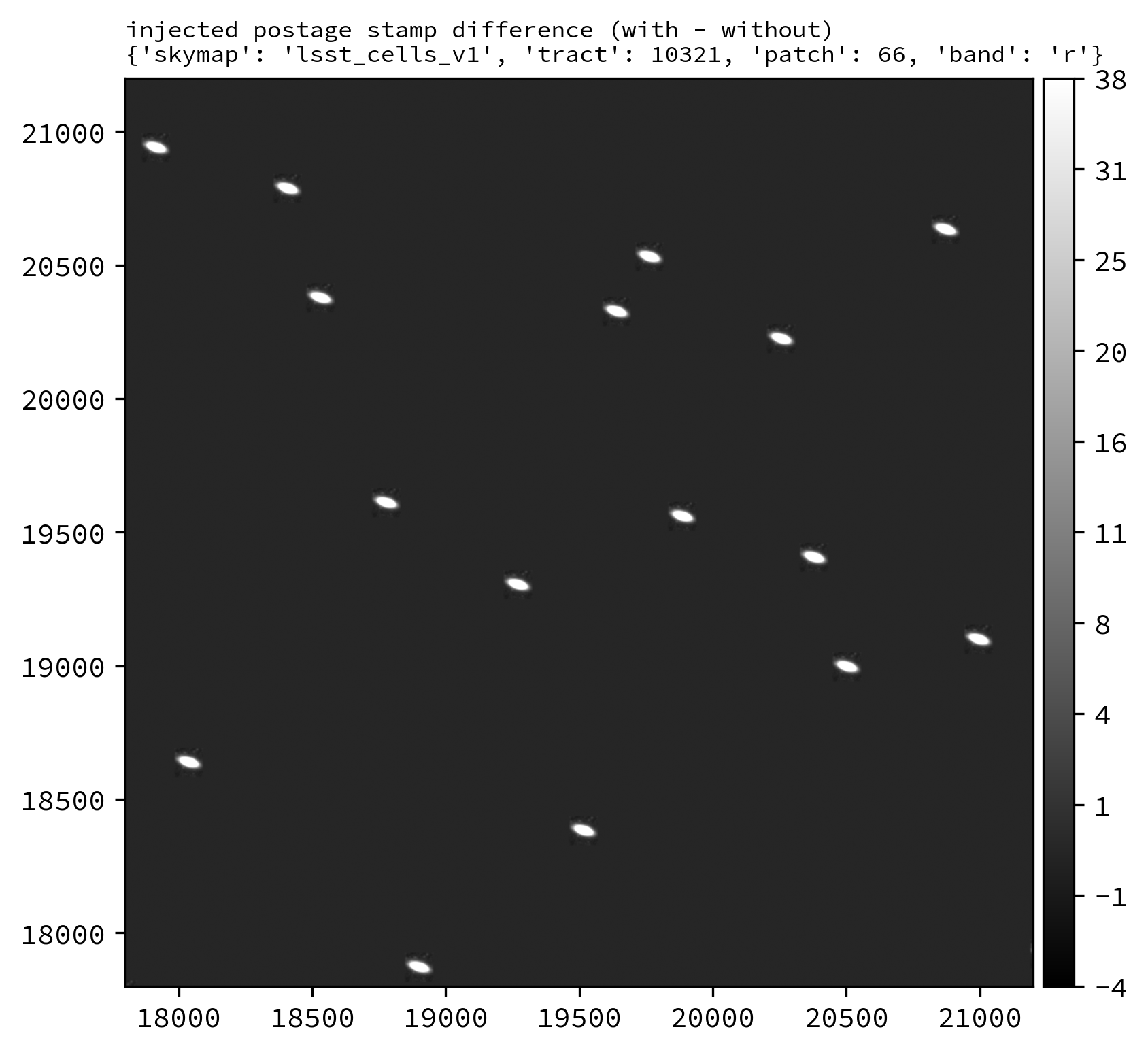
Difference image. |
See also
For a “Rubin themed” example postage stamp injection, see the top of the FAQs page.
Wrap Up#
This page has described how to inject synthetic sources into a visit-level exposure-type or visit-type dataset, or into a coadd-level co-added dataset. Options for injection on the command line and in Python have been presented. The special case of injecting FITS-file postage stamp images has also been covered.
Move on to another quick reference guide, consult the FAQs, or head back to the main page.