WholeTractImage

class lsst.analysis.tools.actions.plot.WholeTractImage(*args, **kw)

Bases: PlotAction

Produces a figure displaying whole-tract coadd pixel data as a 2D image.

The figure is constructed from all patches covering the tract. Regions of NO_DATA or where no coadd exists are shown as red shading or red hatches, respectively.

Either the image, pixel mask, or variance components of the coadd can be displayed. In the case of the pixel mask, one or more bitmaskPlanes must be specified; the specified bitmaskPlanes are OR-combined, with flagged pixels given a value of 1, and unflagged pixels given a value of 1.

Attributes Summary

bitmaskPlanes	List of names of bitmask plane(s) to display when displaying the mask plane.
colorbarCmap	Matplotlib colormap to use for the displayed image.
component	Coadd component to display.
displayAsPostageStamp	Display as a figure to be used as postage stamp.
interval	Action to calculate the min and max values of the image scale.
noDataColor	Matplotlib color to use to indicate regions of no data.
noDataValue	If data doesn't contain a mask plane, the value in the image plane to assign the noDataColor to.
showColorbar	Show a colorbar alongside the main plot.
showPatchIds	Show the patch IDs in the centre of each patch.
stretch	Action to calculate the stretch of the image scale.
vmaxFloor	The floor of the vmax value of the colorbar (float, default None)
zAxisLabel	Label to display on the colorbar.

Methods Summary

__call__(data, **kwargs)	Call self as a function.
getInputSchema()	Return the schema an AnalysisAction expects to be present in the arguments supplied to the __call__ method.
makeFigure(data, tractId, skymap[, plotInfo])	Make a figure displaying the input pixel data.
validate()	Validate the Config, raising an exception if invalid.

Attributes Documentation

bitmaskPlanes

List of names of bitmask plane(s) to display when displaying the mask plane. Bitmask planes are OR-combined. Flagged pixels are given a value of 1; unflagged pixels are given a value of 0. Optional when displaying either the image or variance planes. Required when displaying the mask plane. (List, default None)

colorbarCmap

Matplotlib colormap to use for the displayed image. Default: gray (str, default 'gray')

Allowed values:

'magma'

magma

'inferno'

inferno

'plasma'

plasma

'viridis'

viridis

'cividis'

cividis

'twilight'

twilight

'twilight_shifted'

twilight_shifted

'turbo'

turbo

'berlin'

berlin

'managua'

managua

'vanimo'

vanimo

'Blues'

Blues

'BrBG'

BrBG

'BuGn'

BuGn

'BuPu'

BuPu

'CMRmap'

CMRmap

'GnBu'

GnBu

'Greens'

Greens

'Greys'

Greys

'OrRd'

OrRd

'Oranges'

Oranges

'PRGn'

PRGn

'PiYG'

PiYG

'PuBu'

PuBu

'PuBuGn'

PuBuGn

'PuOr'

PuOr

'PuRd'

PuRd

'Purples'

Purples

'RdBu'

RdBu

'RdGy'

RdGy

'RdPu'

RdPu

'RdYlBu'

RdYlBu

'RdYlGn'

RdYlGn

'Reds'

Reds

'Spectral'

Spectral

'Wistia'

Wistia

'YlGn'

YlGn

'YlGnBu'

YlGnBu

'YlOrBr'

YlOrBr

'YlOrRd'

YlOrRd

'afmhot'

afmhot

'autumn'

autumn

'binary'

binary

'bone'

bone

'brg'

brg

'bwr'

bwr

'cool'

cool

'coolwarm'

coolwarm

'copper'

copper

'cubehelix'

cubehelix

'flag'

flag

'gist_earth'

gist_earth

'gist_gray'

gist_gray

'gist_heat'

gist_heat

'gist_ncar'

gist_ncar

'gist_rainbow'

gist_rainbow

'gist_stern'

gist_stern

'gist_yarg'

gist_yarg

'gnuplot'

gnuplot

'gnuplot2'

gnuplot2

'gray'

gray

'hot'

hot

'hsv'

hsv

'jet'

jet

'nipy_spectral'

nipy_spectral

'ocean'

ocean

'pink'

pink

'prism'

prism

'rainbow'

rainbow

'seismic'

seismic

'spring'

spring

'summer'

summer

'terrain'

terrain

'winter'

winter

'Accent'

Accent

'Dark2'

Dark2

'Paired'

Paired

'Pastel1'

Pastel1

'Pastel2'

Pastel2

'Set1'

Set1

'Set2'

Set2

'Set3'

Set3

'tab10'

tab10

'tab20'

tab20

'tab20b'

tab20b

'tab20c'

tab20c

'grey'

grey

'gist_grey'

gist_grey

'gist_yerg'

gist_yerg

'Grays'

Grays

'magma_r'

magma_r

'inferno_r'

inferno_r

'plasma_r'

plasma_r

'viridis_r'

viridis_r

'cividis_r'

cividis_r

'twilight_r'

twilight_r

'twilight_shifted_r'

twilight_shifted_r

'turbo_r'

turbo_r

'berlin_r'

berlin_r

'managua_r'

managua_r

'vanimo_r'

vanimo_r

'Blues_r'

Blues_r

'BrBG_r'

BrBG_r

'BuGn_r'

BuGn_r

'BuPu_r'

BuPu_r

'CMRmap_r'

CMRmap_r

'GnBu_r'

GnBu_r

'Greens_r'

Greens_r

'Greys_r'

Greys_r

'OrRd_r'

OrRd_r

'Oranges_r'

Oranges_r

'PRGn_r'

PRGn_r

'PiYG_r'

PiYG_r

'PuBu_r'

PuBu_r

'PuBuGn_r'

PuBuGn_r

'PuOr_r'

PuOr_r

'PuRd_r'

PuRd_r

'Purples_r'

Purples_r

'RdBu_r'

RdBu_r

'RdGy_r'

RdGy_r

'RdPu_r'

RdPu_r

'RdYlBu_r'

RdYlBu_r

'RdYlGn_r'

RdYlGn_r

'Reds_r'

Reds_r

'Spectral_r'

Spectral_r

'Wistia_r'

Wistia_r

'YlGn_r'

YlGn_r

'YlGnBu_r'

YlGnBu_r

'YlOrBr_r'

YlOrBr_r

'YlOrRd_r'

YlOrRd_r

'afmhot_r'

afmhot_r

'autumn_r'

autumn_r

'binary_r'

binary_r

'bone_r'

bone_r

'brg_r'

brg_r

'bwr_r'

bwr_r

'cool_r'

cool_r

'coolwarm_r'

coolwarm_r

'copper_r'

copper_r

'cubehelix_r'

cubehelix_r

'flag_r'

flag_r

'gist_earth_r'

gist_earth_r

'gist_gray_r'

gist_gray_r

'gist_heat_r'

gist_heat_r

'gist_ncar_r'

gist_ncar_r

'gist_rainbow_r'

gist_rainbow_r

'gist_stern_r'

gist_stern_r

'gist_yarg_r'

gist_yarg_r

'gnuplot_r'

gnuplot_r

'gnuplot2_r'

gnuplot2_r

'gray_r'

gray_r

'hot_r'

hot_r

'hsv_r'

hsv_r

'jet_r'

jet_r

'nipy_spectral_r'

nipy_spectral_r

'ocean_r'

ocean_r

'pink_r'

pink_r

'prism_r'

prism_r

'rainbow_r'

rainbow_r

'seismic_r'

seismic_r

'spring_r'

spring_r

'summer_r'

summer_r

'terrain_r'

terrain_r

'winter_r'

winter_r

'Accent_r'

Accent_r

'Dark2_r'

Dark2_r

'Paired_r'

Paired_r

'Pastel1_r'

Pastel1_r

'Pastel2_r'

Pastel2_r

'Set1_r'

Set1_r

'Set2_r'

Set2_r

'Set3_r'

Set3_r

'tab10_r'

tab10_r

'tab20_r'

tab20_r

'tab20b_r'

tab20b_r

'tab20c_r'

tab20c_r

'grey_r'

grey_r

'gist_grey_r'

gist_grey_r

'gist_yerg_r'

gist_yerg_r

'Grays_r'

Grays_r

'rocket'

rocket

'rocket_r'

rocket_r

'mako'

mako

'mako_r'

mako_r

'icefire'

icefire

'icefire_r'

icefire_r

'vlag'

vlag

'vlag_r'

vlag_r

'flare'

flare

'flare_r'

flare_r

'crest'

crest

'crest_r'

crest_r

'None'

Field is optional

component

Coadd component to display. Can take one of image, mask, variance. Default: image. (str, default 'image')

Allowed values:

'image'

image

'mask'

mask

'variance'

variance

'None'

Field is optional

displayAsPostageStamp

Display as a figure to be used as postage stamp. No plotInfo or legend is shown, and large fonts are used for axis labels. (bool, default False)

interval

Action to calculate the min and max values of the image scale. Default: Perc. (VectorAction, default <class 'lsst.analysis.tools.actions.plot.calculateRange.Perc'>)

noDataColor

Matplotlib color to use to indicate regions of no data. Default: red (str, default 'red')

noDataValue

If data doesn’t contain a mask plane, the value in the image plane to assign the noDataColor to. Optional. (int, default None)

showColorbar

Show a colorbar alongside the main plot. Default: False (bool, default False)

showPatchIds

Show the patch IDs in the centre of each patch. Default: False (bool, default False)

stretch

Action to calculate the stretch of the image scale. Default: Asinh (TensorAction, default <class 'lsst.analysis.tools.actions.plot.calculateRange.Asinh'>)

vmaxFloor

The floor of the vmax value of the colorbar (float, default None)

zAxisLabel

Label to display on the colorbar. Optional (str, default None)

Methods Documentation

__call__(data: MutableMapping[str, ndarray[tuple[Any, ...], dtype[_ScalarT]] | Scalar | HealSparseMap | Tensor | Mapping], **kwargs) → Mapping[str, Figure] | Figure

Call self as a function.

getInputSchema() → Iterable[tuple[str, type[numpy.ndarray[tuple[Any, ...], numpy.dtype[_ScalarT]]] | type[lsst.analysis.tools.interfaces._interfaces.Scalar] | type[healsparse.healSparseMap.HealSparseMap] | type[lsst.analysis.tools.interfaces._interfaces.Tensor] | type[Mapping]]]

Return the schema an AnalysisAction expects to be present in the arguments supplied to the __call__ method.

Returns:

resultKeyedDataSchema

The schema this action requires to be present when calling this action, keys are unformatted.

makeFigure(data: MutableMapping[str, ndarray[tuple[Any, ...], dtype[_ScalarT]] | Scalar | HealSparseMap | Tensor | Mapping], tractId: int, skymap: BaseSkyMap, plotInfo: Mapping[str, str] | None = None, **kwargs) → Figure

Make a figure displaying the input pixel data.

Parameters:

datalsst.analysis.tools.interfaces.KeyedData

A python dict-of-dicts containing the pixel data to display in the figure. The top level keys are named after the coadd component(s), and must contain at least ‘mask’. The next level keys are named after the patch ID of the coadd component contained as their corresponding value.

tractIdint

Identification number of the tract to be displayed.

skymaplsst.skymap.BaseSkyMap

The sky map used for this dataset. This is referred-to to determine the location of the tract on-sky (for RA and Dec axis ranges) and the location of the patches within the tract.

plotInfodict, optional

A dictionary of information about the data being plotted with keys:

"run"

The output run for the plots (str).

"skymap"

The type of skymap used for the data (str).

"band"

The filter used for this data (str). Optional

"tract"

The tract that the data comes from (str).

Returns:

figmatplotlib.figure.Figure

The resulting figure.

Examples

An example wholeTractImage plot may be seen below:

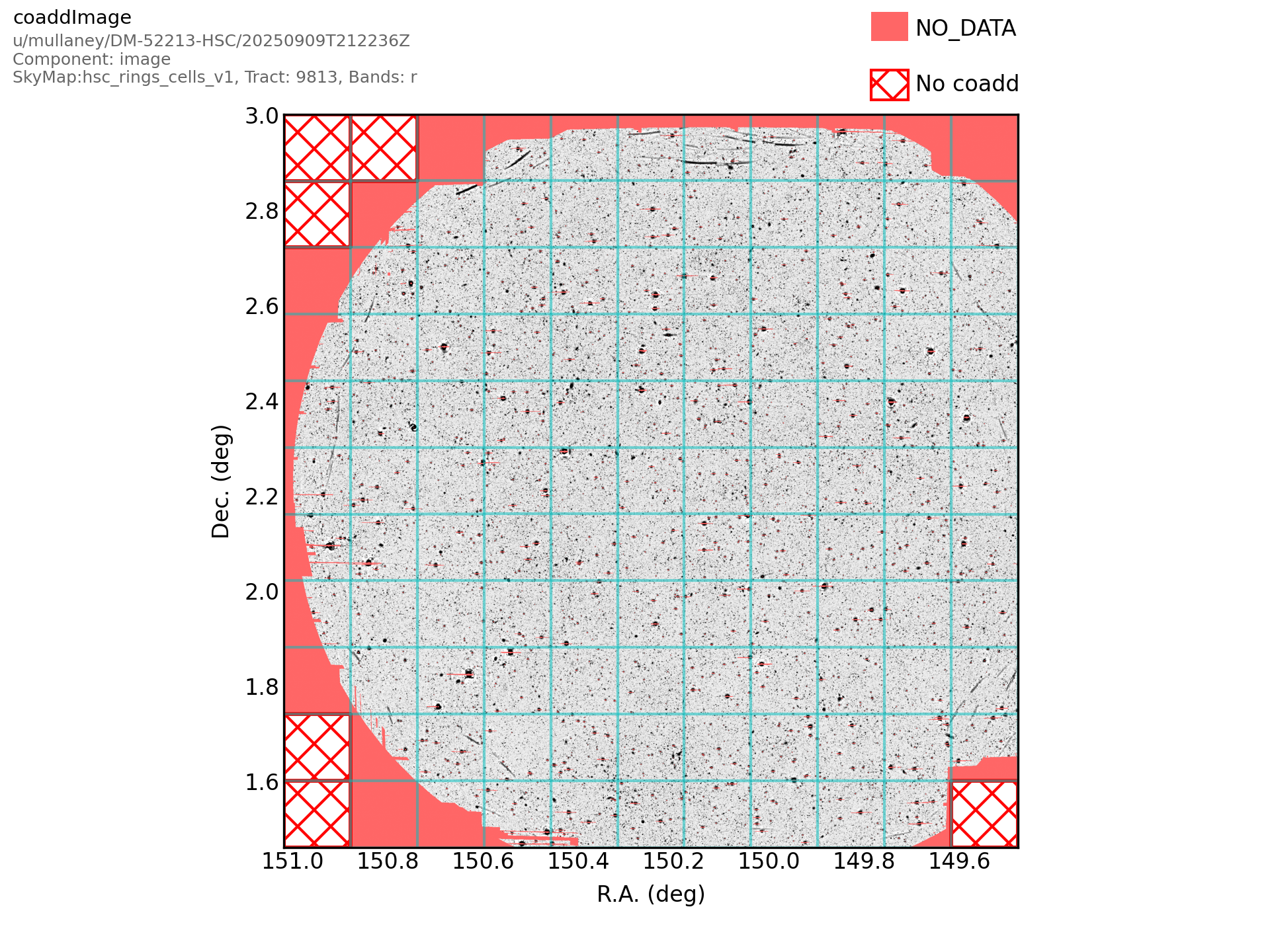
For further details on how to generate a plot, please refer to the getting started guide.

validate()

Validate the Config, raising an exception if invalid.

Raises:

lsst.pex.config.FieldValidationError

Raised if verification fails.

Notes

The base class implementation performs type checks on all fields by calling their validate methods.

Complex single-field validation can be defined by deriving new Field types. For convenience, some derived lsst.pex.config.Field-types (ConfigField and ConfigChoiceField) are defined in lsst.pex.config that handle recursing into subconfigs.

Inter-field relationships should only be checked in derived Config classes after calling this method, and base validation is complete.