Getting started tutorial part 2: calibrating single frames with Pipeline Tasks
In this part of the tutorial series you’ll process individual raw HSC images in the Butler repository (which you assembled in part 1) into calibrated exposures. We’ll use the singleFrame pipeline to remove instrumental signatures with dark, bias and flat field calibration images. This will also use the reference catalog to establish a preliminary WCS and photometric zeropoint solution.
Pipelines are defined in YAML files.
The example git repository contains a pipeline definition for data release processing that is only slightly modified from the one used in production processing of HSC data.
If you are interested in examining the pipeline defintions provided for this tutorial, look in $RC2_SUBSET_DIR/pipelines/DRP.yaml.
Set up
Pick up your shell session where you left off in part 1. For convenience, start in the top directory of the example git repository:
cd $RC2_SUBSET_DIR
The lsst_distrib package also needs to be set up in your shell environment.
See Setting up installed LSST Science Pipelines for details on doing this.
Reviewing what data will be processed
Pipeline tasks can operate on a single image or iterate over multiple images. You can query for the data available to process using the butler command line utility.
butler query-data-ids SMALL_HSC --collections HSC/RC2/defaults --datasets 'raw'
The first few lines look something like:
band instrument detector physical_filter exposure
---- ---------- -------- --------------- --------
   y        HSC       41           HSC-Y      322
   y        HSC       42           HSC-Y      322
   y        HSC       47           HSC-Y      322
   y        HSC       49           HSC-Y      322
Notice the keys that describe each data ID, such as the exposure (exposure identifier for the HSC camera), detector (identifies a specific chip in the HSC camera), band (a generic specifier for about what part of the EM spectrum the filter samples) and physical_filter (the identifier of the specific implementation of this band for the HSC camera).
With these keys you can select exactly what data you want to process.
It’s worth noting that the keys shown here are not the minimal ones needed to specify, for example, a raw.
Only instrument+detector+exposure are necessary to uniquely identify a specific raw dataset, because the system knows that an exposure implies a physical_filter and a physical_filter implies a band.
The raw dataset is special in the sense that it is the starting point for all processing.
Images in the raw dataset have not had any processing applied to them and are as they arrive from the data aquisition system.
The important arguments are --collections and --datasets.
The --collections argument allows you to select which data to search for data IDs.
You can see available collections by, again, using the butler utility.
butler query-collections SMALL_HSC
The --datasets argument allows you to specify what type of data to query for data IDs.
To ask the repository which values are available to pass, you can say:
butler query-dataset-types SMALL_HSC
You can also filter the datasets you get back using the --where argument.
For example, here’s how to select just HSC-I-band datasets:
butler query-data-ids SMALL_HSC --collections HSC/RC2/defaults --datasets 'raw' --where "physical_filter='HSC-I' AND instrument='HSC'"
Now only data IDs for HSC-I datasets are printed.
For instrument specific things like the filter, the instrument must be specified.
The instruments registered with a particular repository can be retrieved using the query-dimension-records subcommand of butler.
E.g.:
butler query-dimension-records SMALL_HSC/ instrument
There is only one instrument in this repository, so you only see metadata about that one instrument. The result of the above command should look like this:
For more information about the butler command line tool, try butler --help.
Running single frame processing
Tip
As mentioned in part 1, this part of the processing is by far the most time consuming.
If you do not wish to process all the data in the repository at this time, you can specify a data query that will reduce the number of exposures to be processed.
Simply add the argument -d "instrument='HSC' AND detector=41 AND exposure=322" to the command line below.
Data queries will be discussed in more detail later.
After learning about datasets, go ahead and run single frame processing using the pipetask command on all raw datasets in the repository:
pipetask run -b $RC2_SUBSET_DIR/SMALL_HSC/butler.yaml \
             -p $RC2_SUBSET_DIR/pipelines/DRP.yaml#singleFrame \
             -i HSC/RC2/defaults \
             -o u/$USER/single_frame \
             --register-dataset-types
There are many arguments to command:pipetask run.
You can get useful information by saying command:pipetask run --help, but let’s go over the ones listed here.
The -b option specifies which butler definition to use when constructing the Butler object to use in processing.
The -p option specifies which pipeline to run.
The full pipeline definition lives in the DRP.yaml file, but subtasks of the full processing can be run by specifying the subtask name with the # character, e.g. #singleFrame in this case.
The -i option indicates the input collections to use in processing.
You will learn more about collections later in this document.
The -o option defines the output collection to send the results of the processing to.
These tutorials suggest that you put the outputs in collections under a namespace defined by your username since that is unique for a given system.
In this case, there is little reason to be so careful because you are likely to have cloned into a space not shared with others.
However, it is good practice for times when you may be using a repository with a registry used by other users on the same system.
The --register-dataset-types switch tells the butler to register a dataset type if it doesn’t already have a definition for it.
Because pipelines are allowed to define datasets at runtime, this switch is necessary if you expect products to be produced that are not already represented in the registry as in this case where we are producing calibrated exposures in a repository that contains only raw files.
If you expect that all of the dataset types should already be registiered, as is the case when processing another subset of data with a pipeline that has already been run, it can help catch unexpected behavior to remove that switch.
Tip
It is not included in the above command, but the -j option is useful if you have more than one core available to you.
Specifying -j<num cores> will run in parallel where <num cores> is the number of processes to execute in parallel.
Dataset queries can be specified using the -d argument to specify which specific datasets should be considered when building the execution graph.
If this argument is omitted, all data in the repository that can be processed based on other inputs, e.g. calibrations, will be.
Aside: collections and quantum graphs
Collections are the primary way data in butler repositories are organized.
Of the types of collections available, the two of interest here are the RUN and CHAINED types.
RUN collections are the least flexible.
Once a dataset is added to a RUN collection, it can never be moved to a different RUN collection.
The constraints on datasets in RUN collections makes these collections that most efficient to store and query.
The collection containing the raw data is a RUN collection.
CHAINED collections are groupings of other collections associated with an alias for that grouping.
The grouping of collections defines the order of collections to search when looking for a dataset associated with a specific data ID.
The collection produced from the -o option above is a CHAINED collection.
The output collection will, in general, include all the collections in the input plus any RUN collections produced by the processing.
The first step of process data is to produce the quantum graph for the processing. This is a directed acyclic graph that completely defines inputs and outputs for every node (quantum) in the graph.
Quantum graphs can be saved for reuse later, and diagnostic graphviz files can be used to visualize the quantum graph.
The qgraph subcommand to pipetask can be used to generate the quantum graph without doing any further processing.
The full processing produces a quantum graph that has many nodes and is hard to look at on one page.
There is a simplified version of the pipeline that is not sufficient for other pipelines, but that does produce a simple enough quantum graph to easily be viewed on one page.
It is called simpleSingleFrame.
Try building the quantum graph for the processing of a single detector:
pipetask qgraph -b $RC2_SUBSET_DIR/SMALL_HSC/butler.yaml \
                -p $RC2_SUBSET_DIR/pipelines/DRP.yaml#simpleSingleFrame \
                -i HSC/RC2/defaults \
                -o u/$USER/single_frame \
                -d "instrument='HSC' AND detector=41 AND exposure=322" \
                --qgraph-dot single_frame.dot \
                --save-qgraph single_frame.qgraph
The quantum graph is saved in pickle format in the file called single_frame.qgraph.
The graphviz file is in single_frame.dot.
If you have graphviz installed, you can turn the dot file into something you look at via a command like this:
dot -Tpdf -osingle_frame.pdf single_frame.dot
This should produce something similar to the following figure.
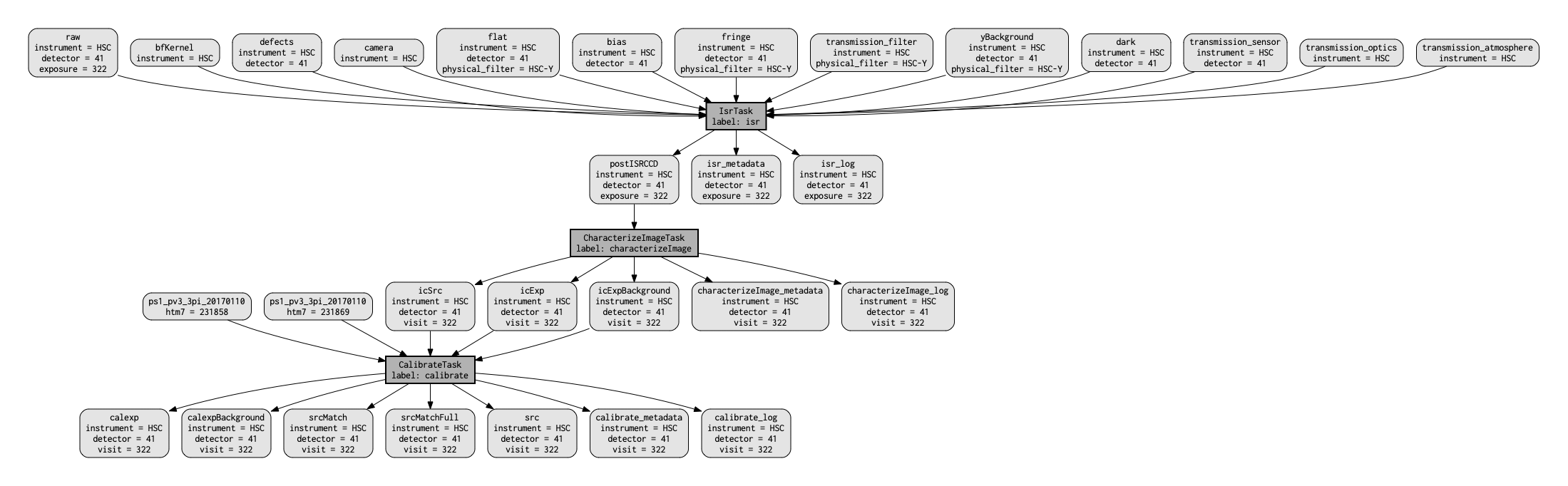
Figure 1 A visualization of the quantum graph generated in this section.
Wrap up
In this tutorial, you’ve used the pipetask run command to calibrate raw images in a Butler repository.
Here are some key takeaways:
- The pipetask run command, with appropriate arguments and switches, processes
rawdatasets, applying both photometric and astrometric calibrations. - Datasets are described by both a type and data ID.
Data IDs are key-value pairs that describe a dataset (for example
filter,visit,ccd,field). - Dataset queries can be used to specify which datasets to process..
- Pipelines write their outputs to a Butler data repository. Collections are used to organize and associate outputs of processing with the inputs to the processing.
Continue this tutorial in part 3, where you’ll learn how to display these calibrated exposures.