Getting started tutorial part 3: displaying exposures and source tables output by single frame processing
In the previous tutorial in the series you used pipetask run configured appropriately to execute the singleFrame pipeline to calibrate a set of raw Hyper Suprime-Cam images.
Now you’ll learn how to use the LSST Science Pipelines to inspect those outputs by displaying images and source catalogs in the DS9 image viewer.
In doing so, you’ll be introduced to some of the LSST Science Pipelines’ Python APIs, including:
- Accessing datasets with the Butler.
- Displaying images in DS9 with
lsst.afw.display. - Working with source catalogs using
lsst.afw.table.
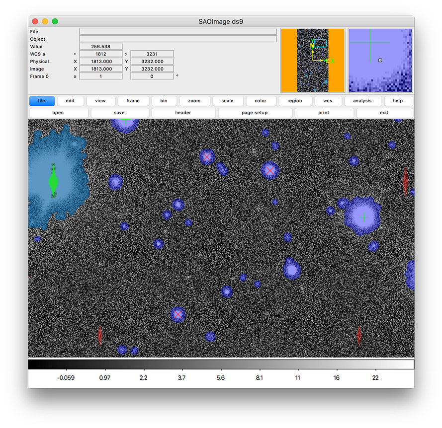
Figure 2 In this tutorial, you’ll create an image display like this one that includes mask planes and source markers.
Set up
Pick up your shell session where you left off in part 2.
For simplicity, the following examples assume your current working directory contains the SMALL_HSC directory (the Butler repository).
cd $RC2_SUBSET_DIR
The lsst_distrib package also needs to be set up in your shell environment.
See Setting up installed LSST Science Pipelines for details on doing this.
You’ll also need to download and install the DS9 image viewer.
Launch DS9 and start a Python interpreter
In this tutorial, you will use an interactive Python session to control DS9. You can also view Science Pipelines image files by loading them directly into DS9, but some features (like color-coded mask planes) will be missing, and many versions of DS9 incorrectly read the mask bits as all zeros.
If you haven’t already, launch the DS9 application.
Next, start up a Python interpreter. You can use the default Python shell (python), the IPython shell, or even run from a Jupyter Notebook. Ensure that this Python session is running from the shell where you ran setup lsst_distrib.
Creating a Butler client
All data in the Pipelines flows through the Butler.
As you saw in the previous tutorial, the singleFrame pipeline reads exposures from the Butler repository and persisted outputs back to the repository.
Although this Butler data repository is a directory on the filesystem (SMALL_HSC), we don’t recommend directly accessing its files.
Instead, you use the Butler client from the lsst.daf.butler module.
In the Python interpreter, run:
from lsst.daf.butler import Butler
butler = Butler('SMALL_HSC')
The Butler client reads from the data repository specified constructor.
In the previous tutorial, you created the single_frame collection to isolate the outputs of singleFrame pipeline.
This collection or a CHAINED collection that contains it will need to be specified whenever accessing datasets it contains.
Tip
By default the Butler constructor returns a read only interface to the repository.
If you plan on adding to the repository, specify writeable=True in the constructor.
Alternatively, if you specify a run to the constructor, it will automatically be writeable and will put outputs into that collection.
Listing available data IDs in the Butler
To get data from the Butler you need to know two things: the dataset type and the data ID.
Every dataset stored by the Butler has a well-defined type.
Pipelines read specific dataset types and output other specific dataset types.
The singleFrame pipeline reads in raw datasets and outputs calexp, or calibrated exposure, datasets (among others).
It’s calexp datasets that you’ll display in this tutorial.
Data IDs let you reference specific instances of a dataset.
You can filter by keys like visit, detector, and physical_filter for raw.
Or keys like exposure, detector, and physical_filter for calexp.
Now, use the Butler client to find what data IDs are available for the calexp dataset type:
import os
collection = f"u/{os.environ['USER']}/single_frame"
for ref in butler.registry.queryDatasets('calexp', physical_filter='HSC-R', collections=collection, instrument='HSC'):
    print(ref.dataId.full)
The printed output are data IDs for the calexp datasets with the HSC-R physical filter.
The collections and instrument arguments are both required in this case.
The first is required because we have not set up default collections to query.
The second is required because we are filtering on an instrument specific key so we need to say which instrument to use since a butler repository can contain data from multiple instruments.
Following are few example lines:
{band: 'r', instrument: 'HSC', detector: 41, physical_filter: 'HSC-R', visit_system: 0, visit: 23718}
{band: 'r', instrument: 'HSC', detector: 42, physical_filter: 'HSC-R', visit_system: 0, visit: 23718}
{band: 'r', instrument: 'HSC', detector: 47, physical_filter: 'HSC-R', visit_system: 0, visit: 23718}
{band: 'r', instrument: 'HSC', detector: 49, physical_filter: 'HSC-R', visit_system: 0, visit: 23718}
{band: 'r', instrument: 'HSC', detector: 50, physical_filter: 'HSC-R', visit_system: 0, visit: 23718}
{band: 'r', instrument: 'HSC', detector: 58, physical_filter: 'HSC-R', visit_system: 0, visit: 23718}
{band: 'r', instrument: 'HSC', detector: 41, physical_filter: 'HSC-R', visit_system: 0, visit: 1214}
{band: 'r', instrument: 'HSC', detector: 42, physical_filter: 'HSC-R', visit_system: 0, visit: 1214}
Note
That example butler.registry.queryDatasets call is similar to this shell command that you used in the previous tutorial.
You can get identical results by specifying a --where argument.
Remember that if you are requesting instrument specific keys, you need to specify which instrument you are interested in.:
butler query-data-ids $RC2_SUBSET_DIR/SMALL_HSC --collections HSC/RC2/defaults --datasets 'raw' --where "physical_filter = 'HSC-R' AND instrument = 'HSC'"
Get an exposure through the Butler
Knowing a specific data ID, let’s get the dataset with the Butler client’s get method:
import os
collection = f"u/{os.environ['USER']}/single_frame"
calexp = butler.get('calexp', visit=23718, detector=41, collections=collection, instrument='HSC')
This calexp is an ExposureF Python object.
Exposures are powerful representations of image data because they contain not only the image data, but also a variance image for uncertainty propagation, a bit mask image plane, and key-value metadata.
In the next steps you’ll learn how to display an Exposure’s image and mask.
Create a display
To display the calexp you will use the display framework, which is imported as:
import lsst.afw.display as afwDisplay
The display framework provides a uniform API for multiple display backends, including DS9 and LSST’s Firefly viewer.
The default backend is ds9, so you can create a display like this:
display = afwDisplay.getDisplay()
Note
You can choose a different backend by setting the backend parameter.
For example:
display = afwDisplay.getDisplay(backend='firefly')
Display the calexp (calibrated exposure)
Then use the display’s mtv method to view the calexp in DS9:
display.mtv(calexp)
Notice that the DS9 display is filled with colorful regions. These are mask regions. Each color reflects a different mask bit that correspond to detections and different types of detector artifacts. You’ll learn how to interpret these colors later, but first you’ll likely want to adjust the image display.
Improving the image display
The display framework gives you control over the image display to help bring out image details.
To make masked regions semi-transparent again, so that underlying image features are visible, try:
display.setMaskTransparency(60)
The setMaskTransparency method’s argument can range from 0 (fully opaque) to 100 (fully transparent).
You can also control the colorbar scaling algorithm with the display’s scale method.
Try an asinh stretch with the zscale algorithm for automatically selecting the white and black thresholds:
display.scale("asinh", "zscale")
Instead of an automatic algorithm like zscale (or minmax) you can explicitly provide both a minimum (black) and maximum (white) value:
display.scale("asinh", -1, 30)
Interpreting displayed mask colors
The display framework renders each plane of the mask in a different color (plane being a different bit in the mask).
To interpret these colors you can get a dictionary of mask planes from the calexp and query the display for the colors it rendered each mask plane with.
Run:
mask = calexp.getMask()
for maskName, maskBit in mask.getMaskPlaneDict().items():
    print('{}: {}'.format(maskName, display.getMaskPlaneColor(maskName)))
As an example, this result is:
BAD: red
CR: magenta
CROSSTALK: None
DETECTED: blue
DETECTED_NEGATIVE: cyan
EDGE: yellow
INTRP: green
NOT_DEBLENDED: None
NO_DATA: orange
SAT: green
SUSPECT: yellow
UNMASKEDNAN: None
Footprints of detected sources are rendered in blue and the saturated cores of bright stars are drawn in green.
Tip
Try customizing the color of a mask plane with the Display.setMaskPlaneColor method.
You can choose any X11 color.
For example:
display.setMaskPlaneColor('DETECTED', 'fuchsia')
display.mtv(calexp)
Getting the source catalog generated by single frame processing
Besides the calibrated exposure (calexp), the singleFrame pipeline also creates a table of the sources it used for PSF estimation as well as astrometric and photometric calibration.
The dataset type of this table is src, which you can get from the Butler:
import os
collection = "u/{os.environ['USER']}/single_frame"
src = butler.get('src', visit=23718, detector=41, collections=collection, instrument='HSC')
This src dataset is a SourceCatalog, which is a catalog object from the lsst.afw.table module.
You’ll explore SourceCatalog objects more in a later tutorial, but you can check its length with Python’s len function:
print(len(src))
The columns of a table are defined in its schema. You can print out the schema to see each column’s name, data type, and description:
print(src.getSchema())
To get just the names of columns, run:
print(src.getSchema().getNames())
To get metadata about a specific column, like calib_psf_used:
print(src.schema.find("calib_psf_used"))
Given a name, you can get a column’s values as a familiar Numpy array like this:
print(src['base_PsfFlux_instFlux'])
Tip
If you are working in a Jupyter notebook you can see an HTML table rendering of any lsst.afw.table table object by getting an astropy.table.Table version of it:
src.asAstropy()
The returned Astropy Table is a view, not a copy, so it doesn’t consume much additional memory.
Plotting sources on the display
Now you’ll overplot sources from the src table onto the image display using the Display’s dot method for plotting markers.
Display.dot plots markers individually, so you’ll need to iterate over rows in the SourceTable.
It’s more efficient to send a batch of updates to the display, though, so enclose the loop in a display.Buffering context, like this:
with display.Buffering():
    for s in src:
        display.dot("o", s.getX(), s.getY(), size=10, ctype="orange")
Now orange circles should appear in the DS9 window over every detected source.
Note
Notice the getX and getY methods for getting the (x,y) centroid of each source.
These methods are shortcuts, using the table’s slot system.
Because the the src catalog contains measurements from several measurement plugins, slots are a way of easily using the pre-configured best measurements of a source.
Clearing markers
Display.dot always adds new markers to the display.
To clear the display of all markers, use the erase method:
display.erase()
Selecting PSF-fitting sources to plot on the display
Next, use the display to understand what sources were used for PSF measurement.
The src table’s calib_psf_used column describes whether the source was used for PSF measurement.
First, set the mask to transparent so it’s easier to see the markers.
Since columns are Numpy arrays we can iterate over rows where src['calib_psf_used'] is True with Numpy’s boolean array indexing:
display.setMaskTransparency(100)
with display.Buffering():
    for s in src[src['calib_psf_used']]:
        display.dot("x", s.getX(), s.getY(), size=10, ctype="red")
Red x symbols on the display mark all stars used by PSF measurement.
Some sources might be considered as PSF candidates, but later rejected.
In this statement, you can use a logical & (and) operator to combine boolean index arrays where both src['calib_psf_candidate'] is True and src['calib_psf_used'] == False as well:
rejectedPsfSources = src[src['calib_psf_candidate'] &
                         (src['calib_psf_used'] == False)]
with display.Buffering():
    for s in rejectedPsfSources:
        display.dot("+", s.getX(), s.getY(), size=10, ctype='green')
Now all green plus (+) symbols on the display mark rejected PSF measurement sources.
The display framework, as you’ve seen, is a useful facility for inspecting images and tables. This tutorial only covered the framework’s basic functionality. Explore the display framework documentation to learn how to display multiple images at once, and to work with different display backends.
A quick look movie
You can use the iterator returned by queryDatasets to make a simple movie, by displaying each calibrated exposure as it is loaded.
import os
from time import sleep
import lsst.afw.display as afwDisplay

display = afwDisplay.getDisplay()
collection = f"u/{os.environ['USER']}/single_frame"
for ref in butler.registry.queryDatasets('calexp', physical_filter='HSC-R', collections=collection, instrument='HSC'):
    calexp = butler.getDirect(ref)
    display.mtv(calexp)
    sleep(1)
Wrap up
In this tutorial you’ve worked with the LSST Science Pipelines Python API to display images and tables. Here are some key takeaways:
- Use the
lsst.daf.butler.Butlerclass to read and write data from repositories. - The
lsst.afw.displaymodule provides a flexible framework for sending data from LSST Science Pipelines code to image displays. You used the DS9 backend in this tutorial, but other backends are available. - Exposure objects have image data, mask data, and metadata. When you display an exposure, the display framework automatically overlays mask planes.
- Tables have well-defined schemas. Use methods like
getSchemato understand the contents of a table. You can also use theasAstropytable method to view the table as anastropy.table.Table.
Continue this tutorial series in part 4, where you’ll produce external calibration products which will be used in coaddition.