

Inspect Injected Outputs#
Visualizing Injected Output Imaging and Examining Output Catalogs#
Once source injection has completed, the source injection task will output two dataset types: an injected image, and an associated injected catalog. The injected image is a copy of the original image with the injected sources added. The injected catalog is a catalog of the injected sources, with the same schema as the original catalog and additional columns describing source injection outcomes.
There are multiple ways to visualize injected output imaging.
The examples on this page make use of the official lsst.afw.display tools for visualization, but other standard visualization tools can also be used, such as those in astropy.visualization.
Visualizing an Injected Image#
First, in Python, lets load an example injected_postISRCCD image produced in Inject Synthetic Sources:
from lsst.daf.butler import Butler

# Instantiate a butler.
butler = Butler.from_config(REPO)

# Load an injected_postISRCCD image.
dataId = dict(
    instrument="LSSTCam",
    exposure=2025050300351,
    detector=94,
)
injected_exposure = butler.get(
    "injected_post_isr_image",
    dataId=dataId,
    collections=OUTPUT_COLL,
)
where
REPOThe path to the butler repository.
OUTPUT_COLLThe name of the injected output collection.
Next lets set up the display, using matplotlib as our backend, and display the image using mtv:
import matplotlib.pyplot as plt
from lsst.afw.display import delAllDisplays, getDisplay, setDefaultBackend

# Set matplotlib as the default backend.
setDefaultBackend("matplotlib")

# Create a figure and a display.
delAllDisplays()
fig = plt.figure(figsize=(6, 8), dpi=300)
display = getDisplay(frame=fig)

# Display the injected_exposure image.
display.mtv(injected_exposure)
Running the above returns something similar to the following:
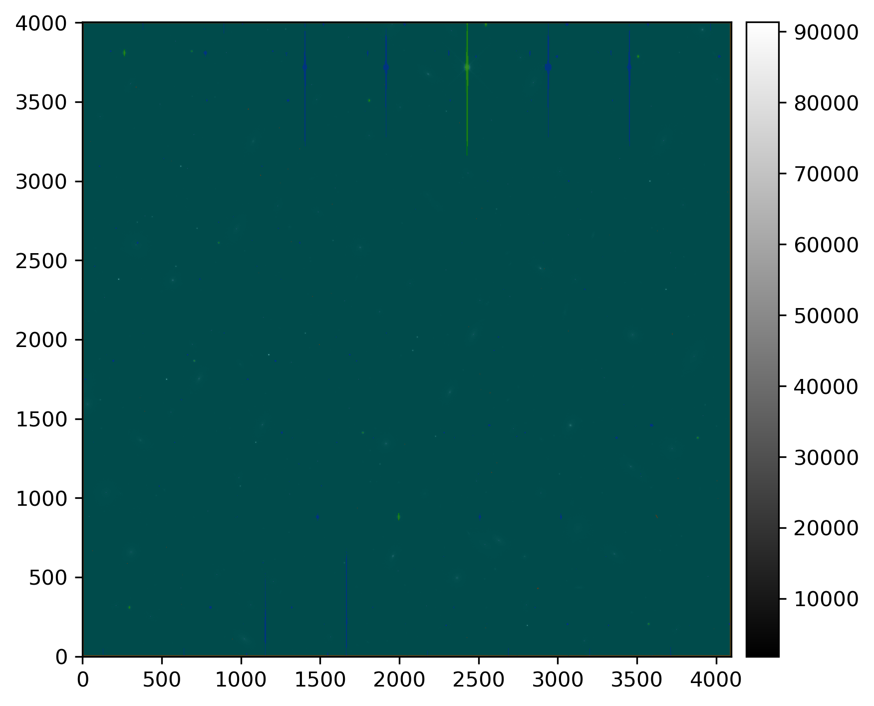
Injected post-ISR image (injected_post_isr_image) for LSSTCam exposure 2025050300351, detector 94, visualized using lsst.afw.display.
Image is scaled using default mtv scaling, with semi-transparent mask planes overlaid.
A number of mask planes of varying color are displayed above.
We can examine the mask attribute for the injected_post_isr_image to determine what each color represents:
.. code-block:: python
# Sort the mask plane dict by bit value and print their mask plane color. mask_plane_dict = injected_exposure.mask.getMaskPlaneDict() sorted_mask_plane_dict = dict(
- sorted(
mask_plane_dict.items(), key=lambda item: item[1],
)
) max_key_length = max(map(len, sorted_mask_plane_dict.keys())) for key in sorted_mask_plane_dict.keys():
print(f”{key: <{max_key_length}} : {display.getMaskPlaneColor(key)}”)
The above returns something similar to:
BAD               : red
SAT               : green
INTRP             : green
CR                : magenta
EDGE              : yellow
DETECTED          : blue
DETECTED_NEGATIVE : cyan
SUSPECT           : yellow
NO_DATA           : orange
VIGNETTED         : red
STREAK            : green
CROSSTALK         : blue
INJECTED          : cyan
INJECTED_CORE     : magenta
ITL_DIP           : yellow
PARTLY_VIGNETTED  : orange
UNMASKEDNAN       : red
Note
The mask plane bit values and colors may vary from one run to another. As such, you should not rely on these values to remain the same between runs.
Note the presence of the INJECTED and INJECTED_CORE mask planes.
These planes have been added by the source injection task.
The INJECTED mask plane shows the draw size for each injected source.
As such, this shows all pixels which were potentially touched by synthetic source injection.
The INJECTED_CORE mask plane shows the central \(3 \times 3\) pixel region of each injected source.
This core region is used to generate an injection flag, which is picked up by downstream data processing tasks to exclude injected sources from consideration for things such as astrometric fitting.
The mtv plotting library is reasonably versatile and can be used to visualize the injected image in a number of ways.
For example, lets mask all mask planes except the INJECTED mask plane, and lets change the scaling for the science image to asinh zscale scaling:
# Create a figure and a display.
delAllDisplays()
fig = plt.figure(figsize=(6, 8), dpi=300)
display = getDisplay(frame=fig)

# Hide all mask planes except INJECTED, using asinh zscale image scaling.
display.setMaskTransparency(100)
display.setMaskTransparency(60, name="INJECTED")
display.scale("asinh", "zscale")

# Display the injected_post_isr_image data.
display.mtv(injected_exposure)
The snippet above returns something similar to:
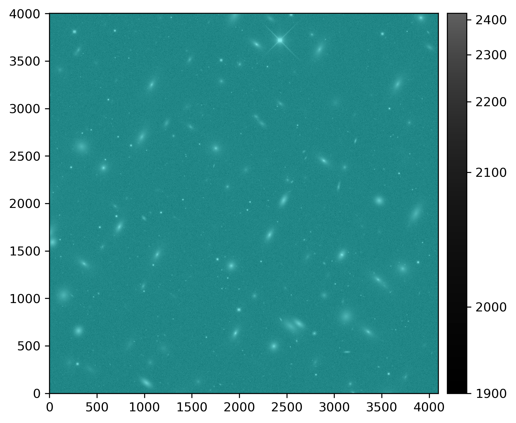
Injected post-ISR image (injected_post_isr_image) for LSSTCam exposure 2025050300351, detector 94, visualized using lsst.afw.display.
Image is asinh zscale scaled, with the INJECTED mask plane shown overlaid.
We can also optionally zoom in to a specific coordinate and highlight the INJECTED_CORE mask plane instead:
# Create a figure and a display.
delAllDisplays()
fig = plt.figure(figsize=(6, 8), dpi=300)
display = getDisplay(frame=fig)

# Show only the INJECTED_CORE mask plane, using asinh zscale scaling.
display.setMaskTransparency(100)
display.setMaskTransparency(60, name="INJECTED_CORE")
display.scale("asinh", "zscale")

# Display the injected_post_isr_image data and zoom in on [1250, 2950].
display.mtv(injected_exposure)
display.zoom(10, 1250, 2950)
The modified snippet above returns something similar to:
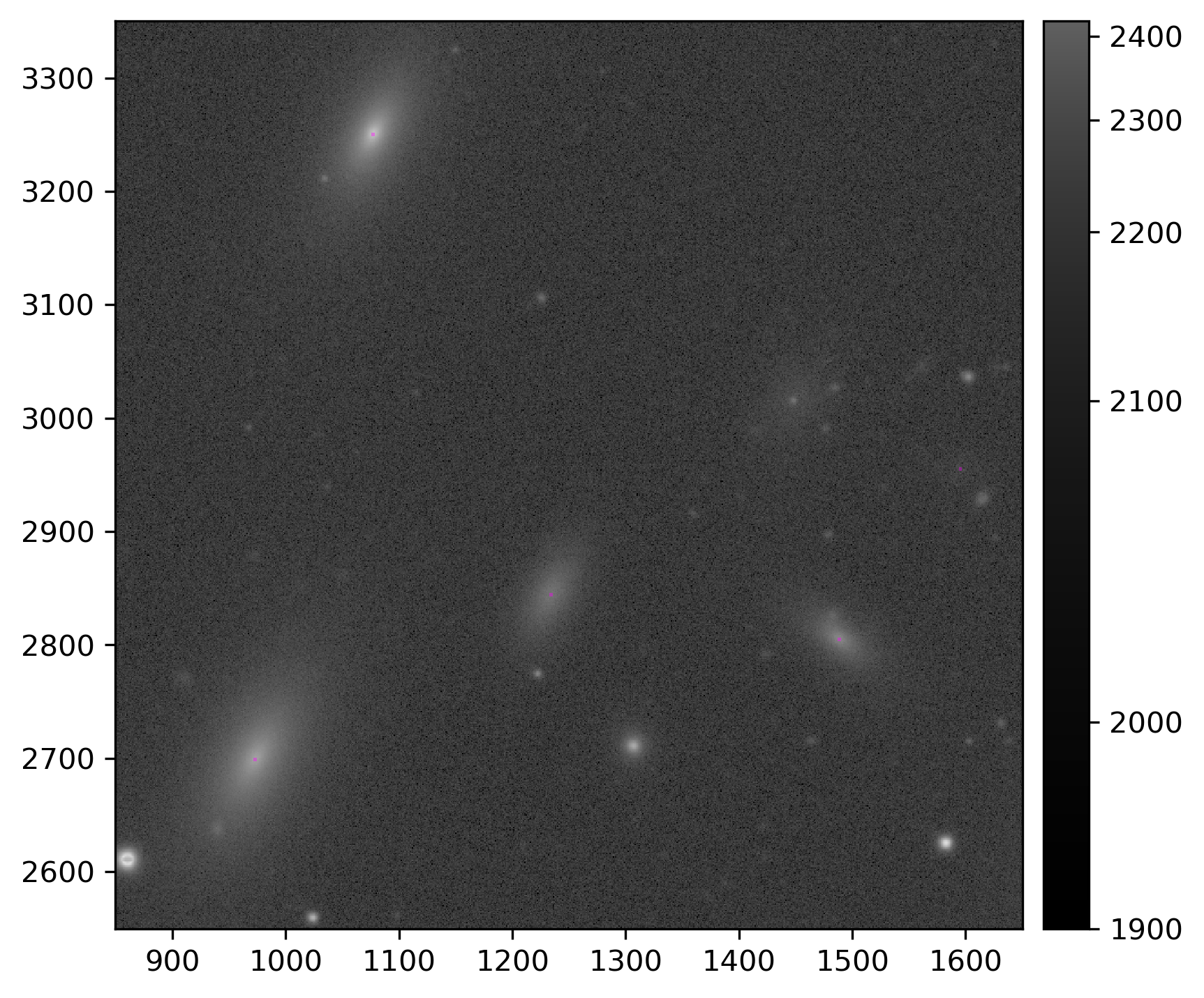
A zoomed in section of an injected post-ISR image (injected_post_isr_image) for LSSTCam exposure 2025050300351, detector 94, visualized using lsst.afw.display.
Image is asinh zscale scaled, with the INJECTED_CORE (magenta) mask plane overlaid.
A difference image can be constructed by subtracting the original image from the injected image:
# Load the original post_isr_image data with the butler.
input_exposure = butler.get(
    "post_isr_image",
    dataId=dataId,
    collections=OUTPUT_COLL,
)

# Subtract the original image from the injected image.
injected_diff = injected_exposure.clone()
injected_diff.image.array = injected_exposure.image.array - input_exposure.image.array

# Create a figure and a display.
delAllDisplays()
fig = plt.figure(figsize=(6, 8), dpi=300)
display = getDisplay(frame=fig)

# Hide all mask planes, and use asinh zscale scaling.
display.setMaskTransparency(100)
display.scale("asinh", "zscale")

# Display the injected difference image.
display.mtv(injected_diff)
where
OUTPUT_COLLThe name of the injected output collection.
The difference image snippet above returns:
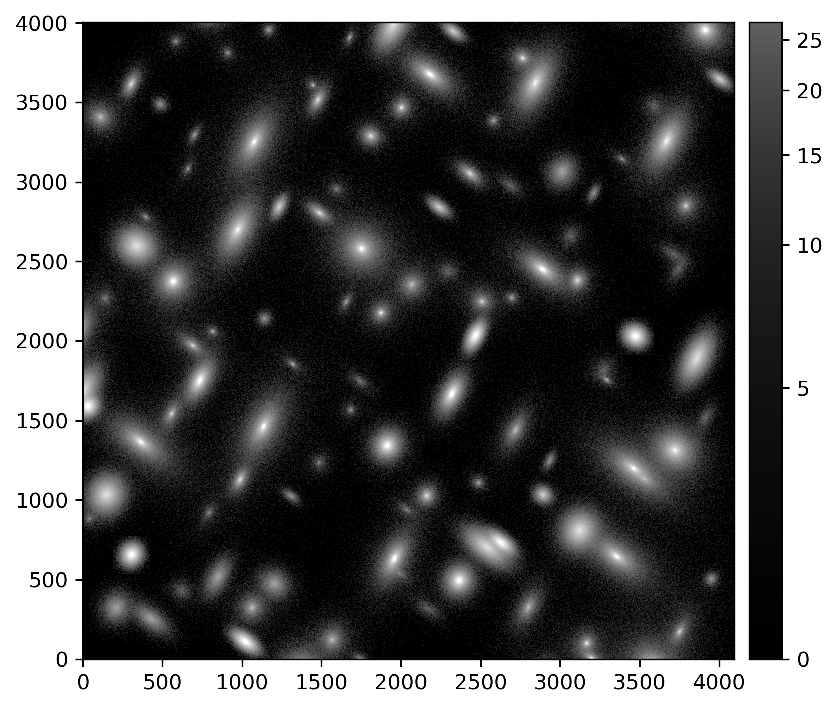
An image showing the difference between an injected post-ISR image (injected_post_isr_image) and a standard post-ISR image (post_isr_image) for LSSTCam exposure 2025050300351, detector 94, visualized using lsst.afw.display.
Image is asinh zscale scaled.
Examine an Injected Catalog#
The source detection task also outputs an injected catalog.
The catalog is named in line with the injected image; for example, an injection into a post_isr_image produces an injected_post_isr_image and an injected_post_isr_image_catalog.
The injected catalog has the same schema as the original catalog, with additional columns providing injection flag information and the draw size (in pixels) associated with the injected source.
The example below loads the associated injected_post_isr_image_catalog for the injected_post_isr_image from above:
.. code-block:: python
from lsst.daf.butler import Butler
# Instantiate a butler. butler = Butler.from_config(REPO)
# Load an injected_post_isr_image catalog. dataId = dict(
instrument=”LSSTCam”, exposure=2025050300351, detector=94,
) injected_catalog = butler.get(
“injected_post_isr_image_catalog”, dataId=dataId, collections=OUTPUT_COLL,
)
where
REPOThe path to the butler repository.
OUTPUT_COLLThe name of the injected output collection.
For this example, this catalog looks like this:
injection_id injection_flag injection_draw_size         ra                dec         source_type mag   n  half_light_radius  q   beta
------------ -------------- ------------------- ------------------ ------------------ ----------- ---- --- ----------------- --- -----
          62              0                 628 185.74127141535553 5.4419263523057895      Sersic 15.0 1.0              10.0 0.5  25.0
          92              0                 472 185.74473093775276  5.376572561793999      Sersic 15.0 2.0               5.0 0.9 125.0
         141              0                1264  185.7223434826212  5.492119251088945      Sersic 15.0 2.0              10.0 0.5  25.0
         142              0                1264 185.70341406475956  5.538522382978416      Sersic 15.0 2.0              10.0 0.5  25.0
         171              0                1314 185.74295452997492  5.550850428274257      Sersic 15.0 4.0               5.0 0.9 125.0
This injected catalog may not be a complete copy of the input catalog. Only sources which stood any chance of being injected are included in the injected catalog. For example, sources which were too far away from the edge of the image to be injected are not included in the injected catalog.
The injection flag value is a binary flag which encodes the outcome of source injection for each source. An injection flag value of 0 indicates that source injection for this source completed successfully. The bit-wise value for all potential flags may be accessed from the metadata attached to the injected catalog:
# Get injection flags from the metadata; print their label and bit value.
injection_flags = injected_catalog.meta
max_key_length = max(map(len, injection_flags.keys()))
for key, value in injection_flags.items():
    print(f"{key: <{max_key_length}} : {value}")
The snippet above returns:
MAG_BAD                         : 0
TYPE_UNKNOWN                    : 1
SERSIC_EXTREME                  : 2
NO_OVERLAP                      : 3
FFT_SIZE_ERROR                  : 4
PSF_COMPUTE_ERROR               : 5
where
MAG_BADThe supplied magnitude was NaN or otherwise non-numeric.
TYPE_UNKNOWNThe
source_typewas not an allowed source type.SERSIC_EXTREMEThe requested Sérsic index was outside the range allowed by GalSim (0.3 < n < 6.2).
NO_OVERLAPWhilst the centroid of the source was close enough to the field of view to be considered for source injection, the draw size was sufficiently small such that no pixels within that bounding box overlap the image.
FFT_SIZE_ERRORA
GalSimFFTSizeErrorwas raised when attempting convolution with the PSF (usually caused by a large requested draw size).PSF_COMPUTE_ERRORA PSF computation error was raised by GalSim.
A source may be flagged for multiple reasons. For example, a source with an invalid magnitude and an unknown source type would have a flag value of \(2^0 + 2^1 = 3\).
Overplot Injected Source Coordinates#
The injected catalog may be used to overplot the coordinates of injected sources on the injected image:
from lsst.daf.butler import Butler

# Assuming the injected data are loaded.

# Get the WCS information from the visit_summary table initially used.
butler = Butler.from_config(REPO)
dataId = dict(
    instrument="LSSTCam",
    visit=2025050300351,
    detector=94,
)
visit_summary = butler.get(
    "visit_summary",
    dataId=dataId,
    collections=INPUT_DATA_COLL,
)
wcs = visit_summary.find(dataId["detector"]).getWcs()

# Get x/y pixel coordinates for injected sources.
xs, ys = wcs.skyToPixelArray(
    injected_catalog["ra"],
    injected_catalog["dec"],
    degrees=True,
)

# Create a figure and a display.
delAllDisplays()
fig = plt.figure(figsize=(6, 8), dpi=300)
display = getDisplay(frame=fig)

# Hide all mask planes, using asinh zscale image scaling.
display.setMaskTransparency(100)
display.scale("asinh", "zscale")

# Display the injected_post_isr_image data.
display.mtv(injected_exposure)

# Overplot injected source centroids.
with display.Buffering():
    for x, y in zip(xs, ys):
        display.dot("o", x, y, size=100, ctype="orange")
where
REPOThe path to the butler repository.
$INPUT_DATA_COLLThe name of the input data collection.
Running the above snippet returns the following figure:
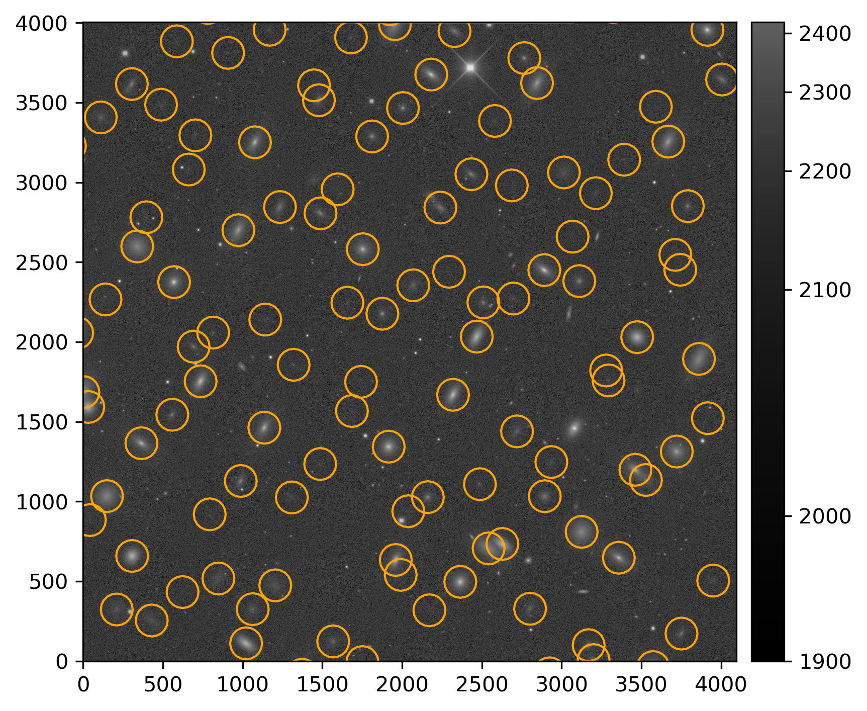
Injected post-ISR image (injected_post_isr_image) for LSSTCam exposure 2025050300351, detector 94, visualized using lsst.afw.display.
Image is asinh zscale scaled.
Injected source centroids are circled in orange.
Wrap Up#
This page has presented methods for visualizing an injected output file and inspecting an injected catalog. Information on how to filter various mask planes during visualization, zoom in on specific regions, highlight sources using their coordinates, construct difference images and determine which sources were successfully injected by using injection flags are discussed.
Move on to another quick reference guide, consult the FAQs, or head back to the main page.