Match Injected Outputs¶

Consolidate and match source injection catalogs¶

This page covers how to match injected input catalogs to output data catalogs. This process can generally be split into two parts: consoliding per-patch injected catalogs into tract-level input catalogs, and matching the input and output catalogs.

Consolidate injected catalogs¶

The butler may split up catalogs which cover multiple photometry bands or which cover large areas of sky for memory efficiency, even when a single catalog is injected. For example, if a coadd-level injected catalog covers a whole tract across multiple photometry bands, the injected catalogs will be split and stored with the dimensions {patch, band}. Before matching the injected input catalogs to the processed output catalog, the per-patch and per-band inputs must be consolidated into a single tract level catalog. This can be done by using pipetask run to run ConsolidateInjectedCatalogsTask from pipelines/consolidate_injected_deepCoadd_catalogs.yaml.

pipetask --long-log --log-file $LOGFILE run \
-b $REPO \
-i $PROCESSED_DATA_COLL \
-o $CONSOLIDATED_CATALOG_COLL \
-p $SOURCE_INJECTION_DIR/pipelines/consolidate_injected_deepCoadd_catalogs.yaml \
-d "instrument='HSC' AND skymap='hsc_rings_v1' AND tract=9813 AND patch=42 AND band='i'"

where

$LOGFILE
The full path to a user-defined output log file.

$REPO
The path to the butler repository.

$PROCESSED_DATA_COLL
The name of the input injected catalog collection.

$CONSOLIDATED_CATALOG_COLL
The name of the consolidated injected output collection.

Matching¶

Now that we have our consolidated tract-level injected catalog and a reference tract-level standard catalog, we can move on to matching these two sets of catalogs together.

The matching tasks are MatchTractCatalogTask and DiffMatchedTractCatalogTask. The first task performs a spatial probablistic match with minimal flag cuts, and the second computes any relevant statistics. These tasks are located in the pipelines/match_injected_tract_catalog.yaml pipeline definition file, with the labels match_object_to_injected and compare_object_to_injected. The pipeline graph for the consolidation and matching process is shown below:

      ○  injected_deepCoadd_catalog
      │
    ○ │  skyMap
    ├─┤
    │ ■  consolidate_injected_catalogs
    │ │
    │ ○  injected_deepCoadd_catalog_tract
    │ │
  ○ │ │  injected_objectTable_tract
╭─┼─┼─┤
■ │ │ │  match_object_to_injected
│ │ │ │
◍ │ │ │  match_target_injected_deepCoadd_catalog_tract_injected_objectTable_tract, match_ref_injected_deepCoadd_catalog_tract_injected_objectTable_tract
╰─┴─┴─┤
      ■  compare_object_to_injected
      │
      ○  matched_injected_deepCoadd_catalog_tract_injected_objectTable_tract

Matching two tract-level catalogs can be done trivially with a pipetask run command as below:

pipetask --long-log --log-file $LOGFILE run \
-b $REPO \
-i $CONSOLIDATED_CATALOG_COLL \
-o $MATCHED_CATALOG_COLL \
-p $SOURCE_INJECTION_DIR/pipelines/match_injected_tract_catalog.yaml \
-d "instrument='HSC' AND skymap='hsc_rings_v1' AND tract=9813 AND patch=42 AND band='i'"

where

$LOGFILE
The full path to a user-defined output log file.

$REPO
The path to the butler repository.

$CONSOLIDATED_CATALOG_COLL
The name of the consolidated injected input collection.

$MATCHED_CATALOG_COLL
The name of the matched injected output collection.

Note

Within pipelines/match_injected_tract_catalog.yaml there are various config options for pre-matching flag selections, columns to copy from the reference and target catalogs, etc.

Visualize the matched catalog and compute metrics¶

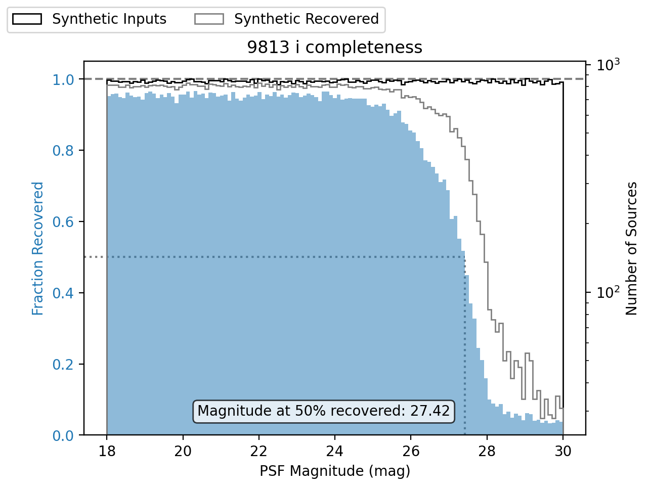
One metric to determine the quality of an injection run is completeness, or the ratio of matched sources to injected sources. The following is an example of a completeness plot using matplotlib.pyplot.

from lsst.daf.butler import Butler
import astropy.units as u
import matplotlib.pyplot as plt
import numpy as np

# Load the matched catalog with the butler.
butler = Butler("/sdf/group/rubin/repo/main")
collections = "u/mccann/DM-41210/RC2"
dtype = "matched_injected_deepCoadd_catalog_tract_injected_objectTable_tract"
tract = 9813
dataId = {"skymap":"hsc_rings_v1", "tract":tract}
data = butler.get(dtype, collections=collections, dataId=dataId)

# Define a matched source flag.
matched = np.isfinite(data["match_distance"])

# Make a completeness plot.
band="i"
flux = f"ref_{band}_flux"
mags = ((data[flux] * u.nJy).to(u.ABmag)).value
fig, axLeft = plt.subplots()
axRight = axLeft.twinx()
axLeft.tick_params(axis="y", labelcolor="C0")
axLeft.set_ylabel("Fraction Recovered", color="C0")
axLeft.set_xlabel("PSF Magnitude (mag)")
axRight.set_ylabel("Number of Sources")
nInput, bins, _ = axRight.hist(
    mags,
    range=(np.nanmin(mags), np.nanmax(mags)),
    bins=121,
    log=True,
    histtype="step",
    label="Synthetic Inputs",
    color="black",
)
nOutput, _, _ = axRight.hist(
    mags[matched],
    range=(np.nanmin(mags[matched]), np.nanmax(mags[matched])),
    bins=bins,
    log=True,
    histtype="step",
    label="Synthetic Recovered",
    color="grey",
)
xlims = plt.gca().get_xlim()
# Find bin where the fraction recovered first falls below 0.5
lessThanHalf = np.where((nOutput / nInput < 0.5))[0]
if len(lessThanHalf) == 0:
    mag50 = np.nan
else:
    mag50 = np.min(bins[lessThanHalf])
    axLeft.plot([xlims[0], mag50], [0.5, 0.5], ls=":", color="grey")
    axLeft.plot([mag50, mag50], [0, 0.5], ls=":", color="grey")
plt.xlim(xlims)
fig.legend(loc="outside upper left", ncol=2)
axLeft.axhline(1, color="grey", ls="--")
axLeft.bar(
    bins[:-1],
    nOutput / nInput,
    width=np.diff(bins),
    align="edge",
    color="C0",
    alpha=0.5,
    zorder=10,
)
bboxDict = dict(boxstyle="round", facecolor="white", alpha=0.75)
info50 = "Magnitude at 50% recovered: {:0.2f}".format(mag50)
axLeft.text(0.3, 0.15, info50, transform=fig.transFigure, bbox=bboxDict, zorder=11)
plt.title(f"{tract} {band} completeness")
fig = plt.gcf()

Completeness for coadd-level matched injected catalog (``matched_injected_deepCoadd_catalog_tract_injected_objectTable_tract``) for HSC tract 9813, ``i`` band, visualized using `matplotlib.pyplot`.

Wrap Up¶

This page has presented methods for consolidating injected catalogs, matching injected inputs with processed outputs, and visualizing a matched catalog. Currently source_injection only supports consolidation and matching for coadd-level injection, but in the future these methods may be generalized for use at the visit and exposure level.

Move on to another quick reference guide, consult the FAQs, or head back to the main page.

Navigation