

Getting Started Guide#
What is analysis_tools?#
Analysis tools is a package for the creation of plots and metrics. It allows them to be created from the same code to ensure that they are consistent and repeatable.
It has powerful and flexible functionality but can be somewhat overwhelming at first. We are going to cover getting the stack set up and cloning analysis_tools. Then an overview of the package and follow that with walking through a series of examples of increasing complexity.
Analysis tools is designed to work with any sort of keyed data but to make it more intuitive initially we’ll talk about tables and column names.
Setting Up the Package and Getting Started With The Stack#
To set up the stack you need to source your version of:
source /opt/lsst/software/stack/loadLSST.bash
and then setup lsst_distrib.
setup lsst_distrib
If you don’t have a local version of analysis_tools but you want to contribute or change things then you can git clone the package from lsst/analysis_tools.
git clone git@github.com:lsst/analysis_tools.git
Once the package has been cloned, it needs to be setup and scons needs to be run to build the package.
setup -j -r repos/analyis_tools
scons repos/analysis_tools
More details can be found here: https://pipelines.lsst.io/install/package-development.html?highlight=github#un-set-up-the-development-package You can check what is set up using this command:
eups list -s
hopefully this will show your local version of analysis_tools.
Package Layout#
There are a bunch of files in analysis_tools but we are going to focus on two directories,
python/lsst/analysis/tools/ and pipelines, which contain the python code and the
pipelines that run it respecitvely. Below is a brief overview of the layout, for more details
please see the package layout guide (still under development).
Pipelines#
visitQualityCore.yaml
The core plots for analysing the quality of the visit level data. The core pipeline is run as standard as part of the regular reprocessing. The most helpful plots go into this pipeline.
visitQualityExtended.yaml
An extended pipeline of plots and metrics to study the visit level data. The extended pipeline is run when a problem comes up or we need to look deeper into the data quality. Useful plots that address specific issues but don’t need to be run on a regular basis get added to this pipeline.
coaddQualityCore.yaml
The core plots for analysing the quality of the coadd level data.
coaddQualityExtended.yaml
The extended plots for analysing the coadd data.
matchedVisitQualityCore.yaml
Plots and metrics that assess the repeatability of sources per tract by matching them between visits.
apDetectorVisitQualityCore.yaml
A metrics pipeline that runs as an afterburner on the butler datasets produced by
ap_pipeon single detector-visits.
python/lsst/analysis/tools#
actions
This contains the actions that plot things and calculate things. Check here before adding new actions to avoid duplication.
scalar
Contains a lot of useful actions that return scalar values. E.g. median or sigma MAD.
vector
These actions run on vectors and return vectors. E.g. the S/N selector which returns an array of bools.
keyedData
These actions are base classes for other actions. You shouldn’t need to add stuff here. Use the scalar or vector actions.
plots
The plotting code lives in here. You shouldn’t need to touch this unless you have to add a new plot type. Try to use one of the existing ones first rather than duplicating things.
atools
Metrics and plots go in here. Similar plots and metrics should be grouped together into the same file, i.e. skyObject.py which contains various plots and metrics that use sky objects.
contexts
Generic settings to be applied in a given circumstance. For example overrides that are specific to a coadd or visit level plot/metric such as the default flag selector which is different between coadd and visit analysis.
interfaces
Interfaces are the framework level code which is used as a basis to build/interact with analysis tools package. You should not have to modify anything in here to be able to add new metrics or plots.
tasks
Each different dataset type requires its own task to handle the reading of the inputs. For example: objectTableTractAnalysis.py which handles the reading in of object tables.
A Simple Plotting And Metric Example#
We will start with a simple example and build up from there. We’re going to start by adapting an existing plot and metric to our needs, we’ll use a sky plot to show the on sky distribution of the values of a column in the table.
The plot/metric is an example of an analysis tool, these are composed of actions which do the actual work of selection and calculation.
We use ‘actions’ to tell the code what to plot on the z axis, these can be defined by anyone but standard ones exist already. This example will showcase some of these standard ones and then we’ll look more into how to define them. One of the great things about actions is that they allow us to only read in the columns we need from large tables.
Each plot and/or metric is its own class, each one has a prep, process and produce section. The prep section manipulates input data, for example by performing flag cuts and signal to noise cuts. The process section builds the data required for the plot/metric, for example if the plot is of a magnitude difference against a magnitude then the actions defined in the process section will identify which flux column needs to be read in and turned into a magnitude. Then another will take the fluxes needed, turn them into magnitudes and then calculate their difference. The produce section takes the prepared and pre calculated data, plots it on the graph and creates the metrics from it. The plot options, such as axis labels, are set in this section.
class newPlotMetric(AnalysisTool):
    def setDefaults(self):
        super().setDefaults()
        self.prep.selectors.flagSelector = CoaddPlotFlagSelector()
        self.prep.selectors.flagSelector.bands = []

        self.prep.selectors.snSelector = SnSelector()
        self.prep.selectors.snSelector.fluxType = "{band}_psfFlux"
        self.prep.selectors.snSelector.threshold = 300

        self.prep.selectors.starSelector = StarSelector()
        self.prep.selectors.starSelector.vectorKey = "{band}_extendedness"

        self.process.buildActions.xStars = LoadVector()
        self.process.buildActions.xStars.vectorKey = "coord_ra"
        self.process.buildActions.yStars = LoadVector()
        self.process.buildActions.yStars.vectorKey = "coord_dec"

        self.process.buildActions.starStatMask = SnSelector()
        self.process.buildActions.starStatMask.fluxType = "{band}_psfFlux"

        self.process.buildActions.zStars = ExtinctionCorrectedMagDiff()
        self.process.buildActions.zStars.magDiff.col1 = "{band}_ap12Flux"
        self.process.buildActions.zStars.magDiff.col2 = "{band}_psfFlux"

        self.process.calculateActions.median = MedianAction()
        self.process.calculateActions.median.vectorKey = "zStars"

        self.process.calculateActions.mean = MeanAction()
        self.process.calculateActions.mean.vectorKey = "zStars"

        self.process.calculateActions.sigmaMad = SigmaMadAction()
        self.process.calculateActions.sigmaMad.vectorKey = "xStars"

        self.produce.plot = SkyPlot()
        self.produce.plot.plotTypes = ["stars"]
        self.produce.plot.plotName = "ap12-psf_{band}"
        self.produce.plot.xAxisLabel = "R.A. (degrees)"
        self.produce.plot.yAxisLabel = "Dec. (degrees)"
        self.produce.plot.zAxisLabel = "Ap 12 - PSF [mag]"
        self.produce.plot.plotOutlines = False

        self.produce.metric.units = {
            "median": "mmag",
            "sigmaMad": "mmag",
            "mean": "mmag"
        }

        self.produce.metric.newNames = {
            "median": "{band}_ap12-psf_median",
            "mean": "{band}_ap12-psf_mean",
            "sigmaMad": "{band}_ap12-psf_sigmaMad",
        }
Let’s look at what the bits do in more detail.
self.prep.selectors.flagSelector = CoaddPlotFlagSelector()
self.prep.selectors.flagSelector.bands = []
The flag selector option lets us apply selectors based on flags to cut the data down. Multiple can be applied at once and any flag that is in the input can be used. However pre built selectors already exist for the common and recommended flag combinations.
CoaddPlotFlagSelector - this is the standard set of flags for coadd plots. The [] syntax means it gets applied in the band the plot is being made in.
self.prep.selectors.snSelector = SnSelector()
self.prep.selectors.snSelector.fluxType = "{band}_psfFlux"
self.prep.selectors.snSelector.threshold = 300
SnSelector - this is the standard way of cutting the data down on S/N, you can set the flux type that is used to calculate the ratio and the threshold which the data must be above to be kept.
self.prep.selectors.starSelector = StarSelector()
self.prep.selectors.starSelector.vectorKey = "{band}_extendedness"
The starSelector option is for defining a selector which picks out the specific type of object that you want to look at. You can define this anyway you want but there are pre defined ones that can be used to choose stars or galaxies. You can also plot both at the same time, either separately or as one dataset but the different dynamic ranges they often cover can make the resulting plot sub optimal.
starSelector - this is the standard selector for stars. It uses the extendedness column, though any column can be specified, the threshold in starSelector is defined for the extendedness column.
self.process.buildActions.xStars = LoadVector()
self.process.buildActions.xStars.vectorKey = "coord_ra"
self.process.buildActions.yStars = LoadVector()
self.process.buildActions.yStars.vectorKey = "coord_dec"
This section, the xStars and yStars options, sets what is plotted on each axis. In this case it is just the column, post selectors applied, that is directly plotted. To do this the LoadVector action is used, it just takes a vectorKey which in this case is the column name. However this can be any action, common actions are already defined but you can define whatever you need and use it here.
self.process.buildActions.starStatMask = SnSelector()
self.process.buildActions.starStatMask.fluxType = "{band}_psfFlux"
The sky plot prints some statistics on the plot, the mask that selects the points to use for these stats is defined by the starStatMask option. In this case it uses a PSF flux based S/N selector.
self.process.buildActions.zStars = ExtinctionCorrectedMagDiff()
self.process.buildActions.zStars.magDiff.col1 = "{band}_ap12Flux"
self.process.buildActions.zStars.magDiff.col2 = "{band}_psfFlux"
The points on the sky plot are color coded by the value defined in the zStars action. Here we have gone for the ExtinctionCorrectedMagDiff, which calculates the magnitude from each of the columns specified as col1 and col2 and then applies extinction corrections and subtracts them. If there is no extinction corrections for the data then it defaults to a straight difference between them.
self.process.calculateActions.median = MedianAction()
self.process.calculateActions.median.vectorKey = "zStars"

self.process.calculateActions.mean = MeanAction()
self.process.calculateActions.mean.vectorKey = "zStars"

self.process.calculateActions.sigmaMad = SigmaMadAction()
self.process.calculateActions.sigmaMad.vectorKey = "zStars"
Next we want to set some metrics, we are going to use the pre calculated zStars values and then calculate their median, mean and sigma MAD as metric values. Later we will rename these so that the names are specific to each band and more informative when displayed.
self.produce.plot = SkyPlot()
self.produce.plot.plotTypes = ["stars"]
self.produce.plot.plotName = "ap12-psf_{band}"
self.produce.plot.xAxisLabel = "R.A. (degrees)"
self.produce.plot.yAxisLabel = "Dec. (degrees)"
self.produce.plot.zAxisLabel = "Ap 12 - PSF [mag]"
self.produce.plot.plotOutlines = False
This section declares the plot type and adds labels and things. We declare that we want to make a sky plot, that plots only objects of type star. Next we give the plot a name that is informative for later identification and add axis labels. The final option specifies if we want patch outlines plotted.
self.produce.metric.units = {
    "median": "mmag",
    "sigmaMad": "mmag",
    "mean": "mmag"
}
We have to set some units for the metrics, these ones are in milli mags.
self.produce.metric.newNames = {
    "median": "{band}_ap12-psf_median",
    "mean": "{band}_ap12-psf_mean",
    "sigmaMad": "{band}_ap12-psf_sigmaMad",
}
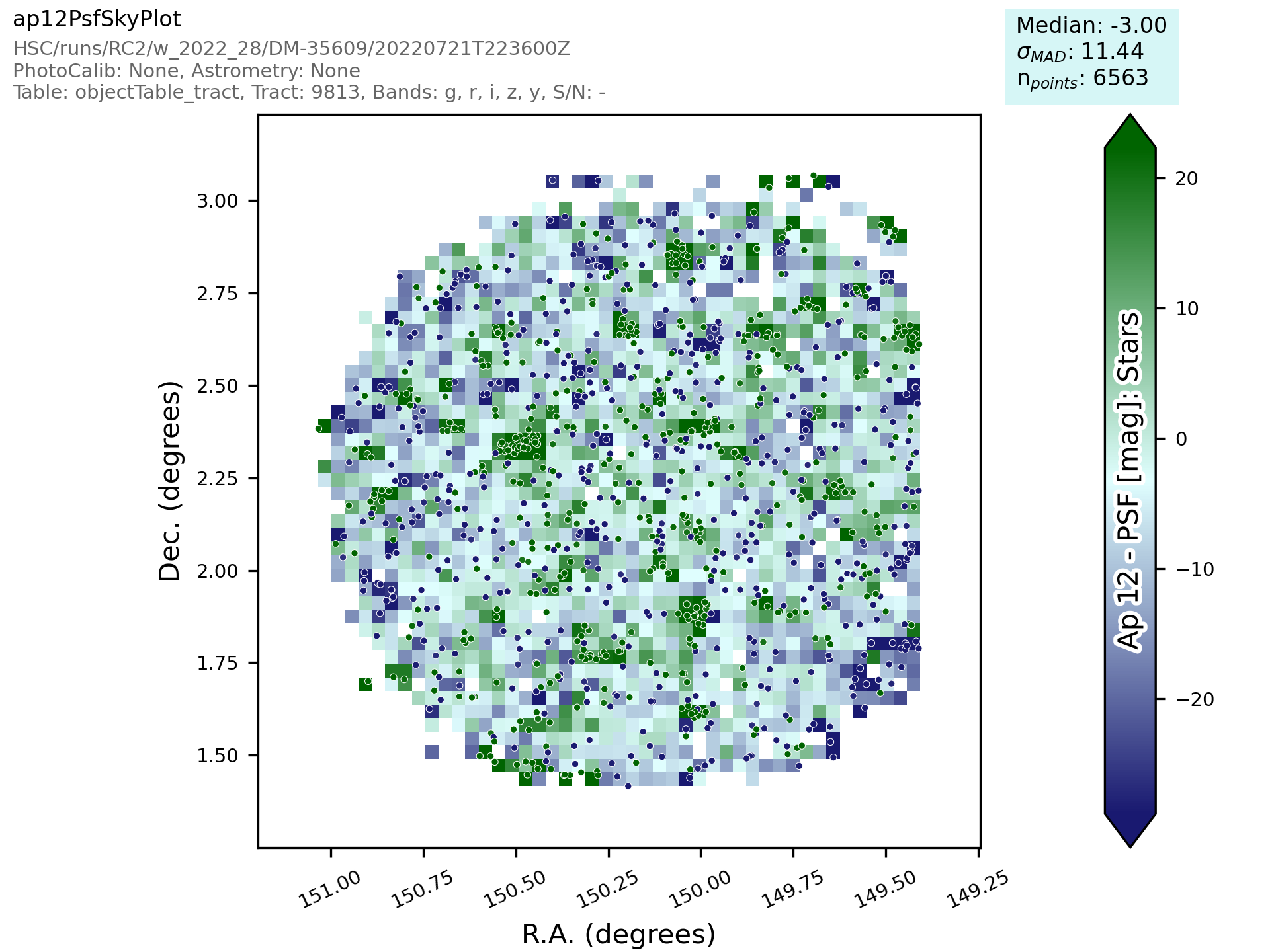
Finally we name the metrics so that the names are specific per band and informative when re-read later. The resulting plot looks a bit like the one here:
This new class then needs to be added to a file in atools, where they go into a file by category, if there isn’t one that suits the tool you are making then start a new file. For example all sky object related plots are in the skyObjects.py file.
Once we have added the class to the relevant file we can now run it from the command line. To do this we need to add the class to a pipeline.
description: |
  An example pipeline to run our new plot
tasks:
  testNewPlot:
  class: lsst.analysis.tools.tasks.ObjectTableTractAnalysisTask
  config:
    connections.outputName: testNewPlot
    plots.newPlot: newPlotMetric
  python: |
    from lsst.analysis.tools.analysisPlots import *
The class line assumes that we want to run the plot on an objectTable_tract. Each different dataset type has its own associated task. Many tasks already exist for different dataset types but depending on what you want to look at you might need to make your own.
Once we have the pipeline we can run it, the same as we would run other pipetasks.
pipetask run -p pipelines/myNewPipeline.yaml
-b /sdf/group/rubin/repo/main/butler.yaml
-i HSC/runs/RC2/w_2022_28/DM-35609
-o u/sr525/newPlotTest
--register-dataset-types --prune-replaced=purge --replace-run
Let’s look at each of the parts that go into the command.
pipetask run -p pipelines/myNewPipeline.yaml
-p is the pipeline file, the location is relative to the directory that the command is run from.
-b /sdf/group/rubin/repo/main/butler.yaml
-b is the location of the butler for the data that you want to process. This example is using the HSC data at the USDF.
-i HSC/runs/RC2/w_2022_28/DM-35609
-i is the input collection to plot from, here we are using one of the weekly reprocessing runs of the RC2 data. This path is relative to the one given for the butler.yaml file in the -b option.
-o u/sr525/newPlotTest
-o is the output collection that you want the plots to go into. The standard way of organising things is to put them into u/your-user-name.
--register-dataset-types --prune-replaced=purge --replace-run
The other options are sometimes necessary when running the pipeline. –register-dataset-types is needed when you have a dataset type that hasn’t been made before and needs to be added. –prune-replaced=purge and –replace-run are useful if you are running the same thing multiple times into the same output, for example when debugging. They replace the previous versions of the plot and just keep the most recent version.
If you don’t want to include all of the data in the input collection then you need to specify a data id which is done with the -d option.
-d "instrument='HSC' AND (band='g' or band='r' or band='i' or band='z' or band='y') AND skymap='hsc_rings_v1'
AND tract=9813 AND patch=68"
This example data id tells the processing that the instrument being used is HSC, that we want to make the plot in the g, r, i, z and y bands, that the skymap used is the hsc_rings_v1 map, that the tract is 9813 and that we only want to process data from patch 68 rather than all the data.
Adding an Action#
Actions go in one of the sub folders of the actions directory depending on what type they are, this is covered in the package layout section. Before you add a new action check if it is already included before adding a duplicate. Sometimes it will probably be better to generalise an exisiting action rather than making a new one that is very similar to something that already exists. If the new action is long or specific to a given circumatance then add it to a new file, for example the ellipticity actions in python/lsst/analysis/tools/actions/vector/ellipticity.py.
The current actions that are available are detailed here. Most common requests are already coded up and please try to reuse actions that already exist before making your own. Please also try to make actions as reusable as possible so that other people can also use them.
Let’s look at some examples of actions. The first one is a scalar action.
class MedianAction(ScalarAction):
    vectorKey = Field[str]("Key of Vector to median.")

    def getInputSchema(self) -> KeyedDataSchema:
        return ((self.vectorKey, Vector),)

    def __call__(self, data: KeyedData, **kwargs) -> Scalar:
        mask = self.getMask(**kwargs)
        return cast(Scalar, float(np.nanmedian(cast(Vector, data[self.vectorKey.format(**kwargs)])[mask])))
Let’s go through what each bit of the action does.
vectorKey = Field[str]("Key of Vector to median.")
This is a config option, when you use the action you declare the column name using this field. This is consistent across all actions.
def getInputSchema(self) -> KeyedDataSchema:
    return ((self.vectorKey, Vector),)
Every action needs a getInputSchema, this is what it uses to know which columns to read in from the table.
This means that only the needed columns can be read in allowing large tables to be accessed without memory
issues. This is one of the bonus benefits of using the `analysis_tools` framework.
def __call__(self, data: KeyedData, **kwargs) -> Scalar:
    mask = self.getMask(**kwargs)
    return cast(Scalar, float(np.nanmedian(cast(Vector, data[self.vectorKey.format(**kwargs)])[mask])))
This actually does the work. It uses a mask, if it is given, and then takes the nan median of the relevant column from the data. The various calls to cast and type declarations are because it is made to work on very generic input data, any sort of keyed data type. Also we’ve got to keep typing happy otherwise we can’t merge to main.
Next we have an example of a vector action, these take vectors and return vectors.
class SubtractVector(VectorAction):
"""Calculate (A-B)"""

    actionA = ConfigurableActionField(doc="Action which supplies vector A", dtype=VectorAction)
    actionB = ConfigurableActionField(doc="Action which supplies vector B", dtype=VectorAction)

    def getInputSchema(self) -> KeyedDataSchema:
        yield from self.actionA.getInputSchema()  # type: ignore
        yield from self.actionB.getInputSchema()  # type: ignore

    def __call__(self, data: KeyedData, **kwargs) -> Vector:
        vecA = self.actionA(data, **kwargs)  # type: ignore
        vecB = self.actionB(data, **kwargs)  # type: ignore

        return vecA - vecB
Vector actions are similar to scalar actions but we will break this one down and look at the components.
actionA = ConfigurableActionField(doc="Action which supplies vector A", dtype=VectorAction)
actionB = ConfigurableActionField(doc="Action which supplies vector B", dtype=VectorAction)
These lines are the config options, here they are the actions which give you the two values to subtract. These actions can be the loadVector action which just reads in a column without changing it in anyway.
def getInputSchema(self) -> KeyedDataSchema:
    yield from self.actionA.getInputSchema()  # type: ignore
    yield from self.actionB.getInputSchema()  # type: ignore
Here we get the column names from each of the actions being used, you can nest actions as deep as you want.
def __call__(self, data: KeyedData, **kwargs) -> Vector:
    vecA = self.actionA(data, **kwargs)  # type: ignore
    vecB = self.actionB(data, **kwargs)  # type: ignore

    return vecA - vecB
This section does the work and calculates the two actions and then subtracts them, returning the results.
These are two very simple examples of actions and how they can be used. They can be as complicated or as simple as you want and can be composed of multiple other actions allowing common segments to be their own actions and then reused.
Adding a Plot Type#
Hopefully there will be very few instances where you will need to add a new plot type and if you do please check open ticket branches to make sure that you are not duplicating someone else’s work. Try to use already existant plot types so that we don’t end up with lots of very similar plot types. Hopefully you won’t really need to touch the plotting code and can just define new classes and actions.
If you add a new plot then please make sure that you include enough providence information on the plot. There should be enough information that anyone can recreate the plot and access the full dataset for further investigation. See the other plots for more information on how to do this. Also please add doc strings to the plot and then add documentation here for other users so that they can easily see what already exists.
The current plot types that are available are detailed here. Most common plots are already coded up and please try to reuse them before making your own. Before adding a new plot type please think about if some of the already coded ones can be adapted to your needs rather than making multiple plots that are basically identical.
numpy and other warnings#
Functions from some external packages such as numpy can issue warnings for e.g. division by zero. These can occur frequently, such as when computing a magnitude from a negative (usually sky-subtracted) flux. numpy warnings do not include a traceback or context and are therefore generally not informative enough to log. Therefore, it is recommended that actions and tasks check for potential issues like NaN values and either log a debug- or info-level message if unexpected values are found, or use the provided mechanisms to filter any uninformative warnings.
There are two built-in methods to filter warnings in analysis_tools:
python/lsst/analysis/tools/math.py contains wrapped version of math functions (from numpy and scipy) that filter warnings so they always result in a particular action. These should be used in place of the standard numpy nan-prefixed functions, unless the action already filters out any values that could produce a warning.
python/lsst/analysis/tools/warning_control.py
has a global setting filterwarnings_action that controls all of the wrapped functions.
This can be set to "error" when debugging new or modified actions and tasks.
python/lsst/analysis/tools/interfaces/_task.py
allows for filtering warnings issued at any other point in task execution, including for direct calls to numpy functions.
Developers can replace the empty list of warnings to catch in _runTools with self.warnings_all or any other list of warning texts.